On July 16th, 1969, 13:32:00 UTC, the Saturn V launch vehicle, SA-506, lifted off from Launch Pad 39-A at Kennedy Space Center, Florida on the Apollo 11 mission with astronauts Neil Armstrong (Mission commander), Michael Collins (Command Module pilot) and Edwin (Buzz) Aldrin (Lunar Module pilot).
L to R: Neil Armstrong, Michael Collins & Buzz Aldrin. Source: NASA
Apollo 11 insignia: Eagle with wings outstretched holding an olive branch above the Moon with Earth in the background.Source: NASA via Wikipedia
The Apollo spacecraft consisted of three modules:
The three-person Command Module (CM), named Columbia, was the living quarters for the three-person crew during most of the lunar landing mission.
The Service Module (SM) contained the propulsion system, electrical fuel cells, consumables storage tanks (oxygen, hydrogen) and various service / support systems.
The two-person, two-stage Lunar Module (LM), named Eagle, would make the Moon landing with two astronauts and return them to the CM.
The LM’s descent stage (bottom part of the LM with the landing legs) remained on the lunar surface and served as the launch pad for the ascent stage (upper part of the LM with the crew compartment). Only the 4.9 ton CM was designed to withstand Earth reentry conditions and return the astronauts safely to Earth.
General configuration of the Apollo spacecraft. The “CSM” is the combined Command Module and Service Module. Source: NASA
From its initial low Earth parking orbit, Apollo 11 flew a direct trans-lunar trajectory to the Moon, inserting into lunar orbit about 76 hours after liftoff. The Apollo 11 mission profile to and from the Moon is shown in the following diagram, and is described in detail here: https://www.mpoweruk.com/Apollo_Moon_Shot.htm
Source: NASA
Neil Armstrong and Buzz Aldrin landed the Eagle LM in the Sea of Tranquility on 20 July 1969, at 20:17 UTC (about 103 hours elapsed time since launch), while Michael Collins remained in a near-circular lunar orbit aboard the CSM. Neil Armstrong characterized the lunar surface at the Tranquility Base landing site with the observation, “it has a stark beauty all its own.”
In the two and a half hours they spent on the lunar surface, Armstrong and Aldrin collected 21.55 kg (47.51 lb) of rock samples, took photographs and set up the Passive Seismic Experiment Package (PSEP) and the Laser Ranging RetroReflector (LRRR), which would be left behind on the Moon. The PSEP provided the first lunar seismic data, returning data for three weeks after the astronauts left, and the LRRR allows precise distance measurements to be collected to this day. Neil Armstrong made an unscheduled jaunt to Little West crater, about 50 m (164 feet) east of the LM, and provided the first view into a lunar crater.
Apollo 11 PSEP in the foreground with astronaut Buzz Aldrin and the LRRR behind it, then the Eagle LM, the American flag, and the TV camera on the left horizon beyond the American flag. Source: NASANeil Armstrong’s photo showing the Eagle LM from Little West crater (33 meters in diameter). Source: NASAApollo 11 landing site captured from 24 km (15 miles) above the surface by NASA’s Lunar Reconnaissance Orbiter (LRO). Source: adapted from NASA Goddard/Arizona State UniversityApollo 11 “traverse” map. Source: NASA via Smithsonian https://airandspace.si.edu/
Armstrong and Aldrin departed the Moon on 21 July 1969 at 17:54 UTC in the ascent stage of the Eagle LM and then rendezvoused and docked with Collins in the CSM about 3-1/2 hours later.
LM Eagle ascent stage with Armstrong and Aldrin approaching the CSM Columbia piloted by Collins. Source: NASA
After discarding the ascent stage, the CSM main engine was fired and Apollo 11 left lunar orbit on 22 July 1969 at 04:55:42 UTC and began its trans-Earth trajectory. As the Apollo spacecraft approached Earth, the SM was jettisoned.
The CM reentered the Earth’s atmosphere and landed in the North Pacific on 24 July 1969 at 16:50:35 UTC. The astronauts and the Apollo 11 spacecraft were recovered by the aircraft carrier USS Hornet. President Nixon personally visited and congratulated the astronauts while they were still in quarantine aboard the USS Hornet. You can watch a video of this meeting here:
Mankind’s first lunar landing mission was a great success.
Postscript to the first Moon landing
A month after returning to Earth, the Apollo 11 astronauts were given a ticker tape parade in New York City, then termed as the largest such parade in the city’s history.
New York City ticker tape parade for the Apollo 11 astronauts. Source: NASA / Bill Taub
There were a total of six Apollo lunar landings (Apollo 11, 12, 14, 15, 16, and 17), with the last mission, Apollo 17, returning to Earth on 19 December 1972. Their landing sites are shown in the following graphic.
The Apollo landing sites. Source: NASA
In the past 46+ years since Apollo 17, there have been no manned missions to the Moon by the U.S. or any other nation.
Along with astronaut John Glenn, the first American to fly in Earth orbit, the three Apollo 11 astronauts were awarded the New Frontier Congressional Gold Medal in the Capitol Rotunda on 16 November 2011. This is the Congress’ highest civilian award and expression of national appreciation for distinguished achievements and contributions.
Neil Armstrong died on 25 August 2012 at the age of 82.
The Apollo 11 command module Columbia was physically transferred to the Smithsonian Institution in 1971 and has been on display for decades at the National Air and Space Museum on the mall in Washington D.C. For the 50th anniversary of the Apollo 11 mission, Columbia will be on display at The Museum of Flight in Seattle, as the star of the Smithsonian Institution’s traveling exhibition, “Destination Moon: The Apollo 11 Mission.” You can get a look at this exhibit at the following link: http://www.collectspace.com/news/news-041319a-destination-moon-seattle-apollo.html
The Apollo 11 command module Columbia at The Museum of Flight in Seattle. Source: collectSPACE
After years of changing priorities under the Bush and Obama administrations, NASA’s current vision for the next U.S. manned lunar landing mission is named Artemis, after the Greek goddess of hunting and twin sister of Apollo. NASA currently is developing the following spaceflight systems for the Artemis mission:
The Space Launch System (SLS) heavy launch vehicle.
A manned “Gateway” station that will be placed in lunar orbit, where it will serve as a transportation node for lunar landing vehicles and manned spacecraft for deep space missions.
The Orion multi-purpose manned spacecraft, which will deliver astronauts from Earth to the Gateway, and also can be configured for deep space missions.
Lunar landing vehicles, which will shuttle between the Gateway and destinations on the lunar surface.
The Orion spacecraft is functionally comparable to the Apollo command and service modules. Source: NASA
While NASA has a tentative goal of returning humans to the Moon by 2024, the development schedules for the necessary Artemis systems may not be able to meet this ambitious schedule. The landing site for the Artemis mission will be in the Moon’s south polar region. NASA administrator Jim Bridenstine has stated that Artemis will deliver the first woman to the Moon.
Robert C. Seamens, Jr., “Project Apollo – The Tough Decisions,” NASA Monographs in Aerospace History Number 37, NASA SP-2007-4537, 2007; https://history.nasa.gov/monograph37.pdf
Ian A. Crawford, “The Scientific Legacy of Apollo,” Astronomy and Geophysics (Vol. 53, pp. 6.24-6.28), December 2012; https://arxiv.org/pdf/1211.6768.pdf
Roger D. Launis, “Apollo’s Legacy: Perspectives on the Moon Landings,” Smithsonian Books, 14 May 2019, ISBN-13: 978-1588346490
Neil Armstrong, Michael Collins & Edwin Aldrin, “First on the Moon,” William Konecky Assoc., 15 October 2002, ISBN-13: 978-1568523989
Michael Collins, “Flying to the Moon: An Astronaut’s Story,” Farrar, Straus and Giroux (BYR); 3 edition, 28 May 2019, ISBN-13: 978-0374312022
Michael Collins, “Carrying the Fire: An Astronaut’s Journeys: 50th Anniversary Edition Anniversary Edition,” Farrar, Straus and Giroux, 16 April 2019, ISBN-13: 978-0374537760
Edwin Aldrin, “Return to Earth,” Random House; 1st edition, 1973, ISBN-13: 978-0394488325
After the failure of Israel’s Beresheet spacecraft to execute a soft landing on the Moon in April 2019, India is the next new contender for lunar soft landing honors with their Chandrayaan-2 spacecraft. We’ll take a look at the Chandrayaan-2 mission in this post.
1. Background: India’s Chandrayaan-1 mission to the Moon
India’s first mission to the Moon, Chandrayaan-1, was a mapping mission designed to operate in a circular (selenocentric) polar orbit at an altitude of 100 km (62 mi). The Chandrayaan-1 spacecraft, which had an initial mass of 1,380 kg (3,040 lb), consisted of two modules, an orbiter and a Moon Impact Probe (MIP). Chandrayaan-1 carried 11 scientific instruments for chemical, mineralogical and photo-geologic mapping of the Moon. The spacecraft was built in India by the Indian Space Research Organization (ISRO), and included instruments from the USA, UK, Germany, Sweden and Bulgaria.
Chandrayaan-1 was launched on 22 October 2008 from the Satish Dhawan Space Center (SDSC) in Sriharikota on an “extended” version of the indigenous Polar Satellite Launch Vehicle designated PSLV-XL. Initially, the spacecraft was placed into a highly elliptical geostationary transfer orbit (GTO), and was sent to the Moon in a series of orbit-increasing maneuvers around the Earth over a period of 21 days. A lunar transfer maneuver enabled the Chandrayaan-1 spacecraft to be captured by lunar gravity and then maneuvered to the intended lunar mapping orbit. This is similar to the five-week orbital transfer process used by Israel’s Bersheet lunar spacecraft to move from an initial GTO to a lunar circular orbit.
The goal of MIP was to make detailed measurements during descent using three instruments: a radar altimeter, a visible imaging camera, and a mass spectrometer known as Chandra’s Altitudinal Composition Explorer (CHACE), which directly sampled the Moon’s tenuous gaseous atmosphere throughout the descent. On 14 November 2008, the 34 kg (75 lb) MIP separated from the orbiter and descended for 25 minutes while transmitting data back to the orbiter. MIP’s mission ended with the expected hard landing in the South Pole region near Shackelton crater at 85 degrees south latitude.
In May 2009, controllers raised the orbit to 200 km (124 miles) and the orbiter mission continued until 28 August 2009, when communications with Earth ground stations were lost. The spacecraft was “found” in 2017 by NASA ground-based radar, still in its 200 km orbit.
Numerous reports have been published describing the detection by the Chandrayaan-1 mission of water in the top layers of the lunar regolith. The data from CHACE produced a lunar atmosphere profile from orbit down to the surface, and may have detected trace quantities of water in the atmosphere. You’ll find more information on the Chandrayaan-1 mission at the following links:
2. India’s upcoming Chandrayaan-2 mission to the Moon
Chandrayaan-2 was launched on 22 July 2019. After achieving a 100 km (62 mile) circular polar orbit around the Moon, a lander module will separate from the orbiting spacecraft and descend to the lunar surface for a soft landing, which currently is expected to occur in September 2019, after a seven-week journey to the Moon. The target landing area is in the Moon’s southern polar region, where no lunar lander has operated before. A small rover vehicle will be deployed from the lander to conduct a 14-day mission on the lunar surface. The orbiting spacecraft is designed to conduct a one-year mapping mission.
Artist’s illustration of India’s lunar lander and the small rover vehicle on the surface of the moon. Source: ISRO
The launch vehicle
India will launch Chandrayaan-2 using the medium-lift Geosynchronous Satellite Launch Vehicle Mark III (GSLV Mk III) developed and manufactured by ISRO. As its name implies, GSLV Mk III was developed primarily to launch communication satellites into geostationary orbit. Variants of this launch vehicle also are used for science missions and a human-rated version is being developed to serve as the launch vehicle for the Indian Human Spaceflight Program.
The GSLV III launch vehicle will place the Chandrayaan-2 spacecraft into an elliptical parking orbit (EPO) from which the spacecraft will execute orbital transfer maneuvers comparable to those successfully executed by Chandrayaan-1 on its way to lunar orbit in 2008. The Chandrayaan-2 mission profile is shown in the following graphic. You’ll find more information on the GSLV Mk III on the ISRO website at the following link: https://www.isro.gov.in/launchers/gslv-mk-iii
Source: ISRO
GSLV Mk III D2 on the launch pad at SDSC for the launchof the GSAT-29 communications satellite in 2018.Source: ISRO via Wikipedia
GSLV Mk III D1 lifting off from the SDSCwith the GSAT-19 communications satellite in 2017.Source: ISRO via WikipediaTransporting the partially integrated GSLV MkIII M1 launch vehicle for the Chandrayaan-2 mission on the Mobile Launch Pedestal. Source: ISRO
The spacecraft
Chandrayaan-2 builds on the design and operating experience from the previous Chandrayaan-1 mission. The new spacecraft developed by ISRO has an initial mass of 3,877 kg (8,547 lb). It consists of three modules: an Orbiter Craft (OC) module, the Vikram Lander Craft (LC) module, and the small Pragyan rover vehicle, which is carried by the LC. The three modules are shown in the following diagram.
Three spacecraft modules (not to scale). Source: ISRO
Chandrayaan-2 carries 13 Indian payloads — eight on the orbiter, three on the lander and two on the rover. In addition, the lander carries a passive Laser Retroreflector Array (LRA) provided by NASA.
Laser Retroreflector Array (LRA). Source: ISRO
The OC and the LC are stacked together within the payload fairing of the launch vehicle and remain stacked until the LC separates in lunar orbit and starts its descent to the lunar surface.
Orbiter (bottom) & lander (top) in stacked configuration. Source: ISRO
The solar-powered orbiter is designed for a one-year mission to map lunar surface characteristics (chemical, mineralogical, topographical), probe the lunar surface for water ice, and map the lunar exosphere using the CHACE-2 mass spectrometer. The orbiter also will relay communication between Earth and Vikram lander.
The orbiter. Source: ISRO
The solar-powered Vikram lander weighs 1,471 kg (3,243 lb). The scientific instruments on the lander will measure lunar seismicity, measure thermal properties of the lunar regolith in the polar region, and measure near-surface plasma density and its changes with time.
The Vikram lander with the Pragyan rover on the ramp.Source: ISRO
The 27 kg (59.5 lb) six-wheeled Pragyan rover, whose name means “wisdom” in Sanskrit, is solar-powered and capable of traveling up to 500 meters (1,640 feet) on the lunar surface. The rover can communicate only with the Vikram lander. It is designed for a 14-day mission on the lunar surface. It is equipped with cameras and two spectroscopes to study the elemental composition of lunar soil.
Rover during testing. Source: ISRORover details. Source: ISRO
You’ll find more information on the spacecraft in the 2018 article by V. Sundararajan, “Overview and Technical Architecture of India’s Chandrayaan-2 Mission to the Moon,” at the following link:
Best wishes to the Chandrayaan-2 mission team for a successful soft lunar landing and long-term lunar mapping mission.
Update 2 December 2019: Vikram lander crashed on the Moon
After a 48-day transit following launch, and an apparently nominal descent toward the lunar surface, communications with the Vikram lander were lost on 6 September 2019, when the spacecraft was at an altitude of about 2 km (1.2 miles), with just seconds remaining before the planned landing. Communications with the Chandrayaan orbiter continued after communications was lost with the Vikram lander. More details on India’s failed landing attempt are in the 25 November 2019 article on the Space.com website here: https://www.space.com/india-admits-moon-lander-crash.html
The firm Northrop Grumman Innovation Systems (formerly Orbital ATK, and before that, Orbital Sciences Corporation) was the first to develop a commercial, air-launched rocket capable of placing payloads into Earth orbit. Initial tests of their modest-size Pegasus launch vehicle were made in 1990 from the NASA B-52 that previously had been used as the “mothership” for the X-15 experimental manned space plane and many other experimental vehicles.
Since 1994, Orbital ATK has been using a specially modified civilian Lockheed L-1011 TriStar, a former airliner renamed Stargazer, as a mothership to carry a Pegasus launch vehicle to high altitude, where the rocket is released to fly a variety of missions, including carrying satellites into orbit. With a Pegasus XL as its payload (launch vehicle + satellite), Stargazer is lifting up to 23,130 kg (50,990 pounds) to a launch point at an altitude of about 12.2 km (40,000 feet).
Orbital ATK’s Pegasus XL rocket released from Stargazer. Source: NASA / http://mediaarchive.ksc.nasa.gov
Paul Allen’s firm Stratolaunch Systems Corporation (https://www.stratolaunch.com) was founded in 2011 to take this air-launch concept to a new level with their giant, twin-fuselage, six-engine Stratolaunch carrier aircraft. The aircraft has a wingspan of 385 feet (117 m), which is the greatest of any aircraft ever built, a length of 238 feet (72.5 m), and a height of 50 feet (15.2 m) to the top of the vertical tails. The empty weight of the aircraft is about 500,000 pounds (226,796 kg). It is designed for a maximum takeoff weight of 1,300,000 pounds (589,670 kg), leaving about 550,000 pounds (249,486 kg) for its payload and the balance for fuel and crew. It will be able to carry multiple launch vehicles on a single mission to a launch point at an altitude of about 35,000 feet (10,700 m). A mission profile for the Stratolaunch aircraft is shown in the following diagram.
Typical air-launch mission profile. Source: Stratolaunch Systems
Stratolaunch rollout – 2017
Built by Scaled Composites, the Stratolaunch aircraft was unveiled on 31 May 2017 when it was rolled out at the Mojave Air and Space Port in Mojave, CA. Following is a series of photos from Stratolaunch Systems showing the rollout.
Stratolaunch ground tests – 2017 to 2019
Ground testing of the aircraft systems started after rollout. By mid-September 2017, the first phase of engine testing was completed, with all six Pratt & Whitney PW4000 turbofan engines operating for the first time. The first low-speed ground tests conducted in December 2017 reached a modest speed of 25 knot (46 kph). By January 2019, the high-speed taxi tests had reached a speed of about 119 knots (220 kph) with the nose wheel was off the runway, almost ready for lift off. Following is a series of photos from Stratolaunch Systems showing the taxi tests.
Stratolaunch first flight
The Stratolaunch aircraft, named Roc, made an unannounced first flight from the Mojave Air & Space Port on 13 April 2019. The aircraft stayed aloft for 2.5 hours, reached a peak altitude of 17,000 feet (5,180 m) and a top speed of 189 mph (304 kph). The following series of photos show the Stratolaunch aircraft during its first flight.
Source, above two photos: Stratolaunch SystemsSource: REUTERS/Gene Blevins/File PhotoLanding at the conclusion of the first flight. Source: Stratolaunch Systems
Stratolaunch posted an impressive short video of the first flight, which you can view here:
Stratolaunch family of launch vehicles: ambitious plans, but subject to change
In August 2018, Stratolaunch announced its ambitious launch vehicle development plans, which included the family of launch vehicles shown in the following graphic:
Up to three Pegasus XL launch vehicles from Northrop Grumman Innovation Systems (formerly Orbital ATK) can be carried on a single Stratolaunch flight. Each Pegasus XL is capable of placing up to 370 kg (816 lb) into a low Earth orbit (LEO, 400 km / 249 mile circular orbit).
Medium Launch Vehicle (MLV) capable of placing up to 3,400 kg (7,496 lb) into LEO and intended for short satellite integration timelines, affordable launch and flexible launch profiles. MLV was under development and first flight was planned for 2022.
Medium Launch Vehicle – Heavy, which uses three MLV cores in its first stage. That vehicle would be able to place 6,000 kg (13,228 lb) into LEO. MLV-Heavy was in the early development stage.
A fully reusable space plane named Black Ice, initially intended for orbital cargo delivery and return, with a possible follow-on variant for transporting astronauts to and from orbit. The space plane was a design study.
Stratolaunch was developing a 200,000 pound thrust, high-performance, liquid fuel hydrogen-oxygen rocket engine, known as the “PGA engine”, for use in their family of launch vehicles. Additive manufacturing was being widely used to enable rapid prototyping, development and manufacturing. Successful tests of a 100% additive manufactured major subsystem called the hydrogen preburner were conducted in November 2018.
Stratolaunch Systems planned family of launch vehicles announced in August 2018. Source: Stratolaunch Systems
After Paul Allen’s death on 15 October 2018, the focus of Stratolaunch Corp was greatly revised. On 18 January 2019, the company announced that it was ending work on its own family of launch vehicles and the PGA rocket engine. The firm announced, “We are streamlining operations, focusing on the aircraft and our ability to support a demonstration launch of the Northrop Grumman Pegasus XL air-launch vehicle.”
You’ll find an article describing Stratolaunch Systems’ frequently changing launch vehicle plans in an article on the SpaceNews website here:
Air launch offers a great deal of flexibility for launching a range of small-to-medium sized satellites and other aerospace vehicles. With only the Pegasus XL as a launch vehicle, and with Northrop Grumman having their own Stargazer carrier aircraft for launching the Pegasus XL, the business case for the Stratolaunch aircraft has been greatly weakened.
Stratolaunch’s main competition: The Northrop Grumman Stargazer at the Mojave Air and Space Port in January 2019, available for its next Pegasus XL launch mission. Source: Author’s photo
Additional competition in the airborne launch services business will come in 2020 from Richard Branson’s firm Virgin Orbit, with its airborne launch platform Cosmic Girl, a highly-modified Boeing 747, and its own launch vehicle, known as LauncherOne. Successful drop tests of LauncherOne were conducted in 2019. The first launch to orbit is expected to occur in 2020. You’ll find more information on the Virgin Orbit website here: https://virginorbit.com
An inert LauncherOne rocket falls away from its 747 carrier aircraft in a July 2019 drop test. Source: Virgin Orbit
Additional competition for small satellite launch services comes from the newest generation of small orbital launch vehicles, like Electron (Rocket Lab, New Zealand) and Prime (Orbix, UK), which are expected to offer low price launch services from fixed land-based launch sites. Electron is operational now, and achieved six successful launches in six attempts in 2019. Prime is expected to enter service in 2021.
In the cost competitive launch services market, Stratolaunch does not seem to have an advantage with only the Pegasus XL in its launch vehicle inventory. Hopefully, they have something else up their sleeve that will take advantage of the remarkable capabilities of the Stratolaunch carrier aircraft.
19 March 2020 Update: Stratolaunch change of ownership
Several sources reported on 11 October 2019 that Stratolaunch Systems had been sold by its original holding company, Vulcan Inc., to an undisclosed new owner. Two months later, Mark Harris, writing for GeekWire, broke the news that the private equity firm Cerberus Capital Management was the new owner. It appears that Jean Floyd, Stratolaunch’s president and CEO since 2015, remains in his roles for now. Michael Palmer, Cerberus’ managing director, was named Stratolaunch’s executive vice president. You can read Mark Harris’ report here: https://www.geekwire.com/2019/exclusive-buyer-paul-allens-stratolaunch-space-venture-secretive-trump-ally/
It will be interesting to watch as the new owners reinvent Stratolaunch Systems for the increasingly competitive market for airborne launch services.
Since late August 2017, the US LIGO 0bservatories in Washington and Louisiana and the European Gravitational Observatory (EGO), Virgo, in Italy, have been off-line for updating and testing. These gravitational wave observatories were set to start Observing Run 3 (O3) on 1 April 2019 and conduct continuous observations for one year. All three of these gravitational wave observatories have improved sensitivities and are capable of “seeing” a larger volume of the universe than in Observing Run 2 (O2).
Later in 2019, the Japanese gravitational wave observatory, KAGRA, is expected to come online for the first time and join O3. By 2024, a new gravitational wave observatory in India is expected to join the worldwide network.
On the advent of this next gravitational wave detection cycle, here’s is a brief summary of the status of worldwide gravitational wave observatories.
Advanced LIGO
The following upgrades were implemented at the two LIGO observatories since Observing Run 2 (O2) concluded in 2017:
Laser power has been doubled, increasing the detectors’ sensitivity to gravitational waves.
Upgrades were made to LIGO’s mirrors at both locations, with five of eight mirrors being swapped out for better-performing versions.
Upgrades have been implemented to reduce levels of quantum noise. Quantum noise occurs due to random fluctuations of photons, which can lead to uncertainty in the measurements and can mask faint gravitational wave signals. By employing a technique called quantum “squeezing” (vacuum squeezing), researchers can shift the uncertainty in the laser light photons around, making their amplitudes less certain and their phases, or timing, more certain. The timing of photons is what is crucial for LIGO’s ability to detect gravitational waves. This technique initially was developed for gravitational wave detectors at the Australian National University, and matured and routinely used since 2010 at the GEO600 gravitational wave detector in Hannover, Germany,
In comparison to its capabilities in 2017 during O2, the twin LIGO detectors have a combined increase in sensitivity of about 40%, more than doubling the volume of the observable universe.
You’ll find more news and information on the LIGO website at the following link:
GEO600 is a modest-size laser interferometric gravitational wave detector (600 meter / 1,969 foot arms) located near Hannover, Germany. It was designed and is operated by the Max Planck Institute for Gravitational Physics, along with partners in the United Kingdom.
In mid-2010, GEO600 became the first gravitational wave detector to employ quantum “squeezing” (vacuum squeezing) and has since been testing it under operating conditions using two lasers: its standard laser, and a “squeezed-light” laser that just adds a few entangled photons per second but significantly improves the sensitivity of GEO600. In a May 2013 paper entitled, “First Long-Term Application of Squeezed States of Light in a Gravitational Wave Observatory,” researchers reported the following results of operational tests in 2011 and 2012.
“During this time, squeezed vacuum was applied for 90.2% (205.2 days total) of the time that science-quality data were acquired with GEO600. A sensitivity increase from squeezed vacuum application was observed broadband above 400 Hz. The time average of gain in sensitivity was 26% (2.0 dB), determined in the frequency band from 3.7 to 4.0 kHz. This corresponds to a factor of 2 increase in the observed volume of the Universe for sources in the kHz region (e.g., supernovae, magnetars).”
The installed GEO600 squeezer (in the foreground) inside the GEO600 clean room together with the vacuum tanks (in the background). Source: http://www.geo600.org/15581/1-High-Tech
While GEO600 has conducted observations in coordination with LIGO and Virgo, GEO600 has not reported detecting gravitational waves. At high frequencies GEO600 sensitivity is limited by the available laser power. At the low frequency end, the sensitivity is limited by seismic ground motion.
You’ll find more information on GEO600 at the following link:
Advanced Virgo, the European Gravitational Observatory (EGO)
At Virgo, the following upgrades were implemented since Observing Run 2 (O2) concluded in 2017:
The steel wires used during O2 observation campaign to suspend the four main mirrors of the interferometer have been replaced. The 42 kg (92.6 pound) mirrors now are suspended with thin fused-silica (glass) fibers, which are expected to increase the sensitivity in the low-medium frequency region. The mirrors in Advanced LIGO have been suspended by similar fused-silica fibers since those two observatories went online in 2015.
A more powerful laser source has been installed, which should improve sensitivity at high frequencies.
Quantum “squeezing” has been implemented in collaboration with the Albert Einstein Institute in Hannover, Germany. This should improve the sensitivity at high frequencies.
Virgo mirror suspension with fused-silica fibers. Source: EGO/Virgo Collaboration/Perciballi
In comparison to its capabilities in 2017 during O2, Virgo sensitivity has been improved by a factor of about 2, increasing the volume of the observable universe by a factor of about 8.
You’ll find more information on Virgo at the following link:
KAGRA is a cryogenically-cooled laser interferometer gravitational wave detector that is sited in a deep underground cavern in Kamioka, Japan. This gravitational wave observatory is being developed by the Institute for Cosmic Ray Research (ICRR) of the University of Tokyo. The project website is at the following link:
One leg of the KAGRA interferometer. Source: ICRR, University of Tokyo
The cryogenic mirror cooling system is intended to cool the mirror surfaces to about 20° Kelvin (–253° Celsius) to minimize the motion of molecules (jitter) on the mirror surface and improve measurement sensitivity. KAGRA’s deep underground site is expected to be “quieter” than the LIGO and VIRGO sites, which are on the surface and have experienced effects from nearby vehicles, weather and some animals.
The focus of work in 2018 was on pre-operational testing and commissioning of various systems and equipment at the KAGRA observatory. In December 2018, the KAGRA Scientific Congress reported that, “If our schedule is kept, we expect to join (LIGO and VIRGO in) the latter half of O3…” You can follow the latest news from the KAGRA team here:
IndIGO, the Indian Initiative in Gravitational-wave Observations, describes itself as an initiative to set up advanced experimental facilities, with appropriate theoretical and computational support, for a multi-institutional Indian national project in gravitational wave astronomy. The IndIGO website provides a good overview of the status of efforts to deploy a gravitational wave detector in India. Here’s the link:
On 22 January 2019, T. V. Padma reported on the Naturewebsite that India’s government had given “in-principle” approval for a LIGO gravitational wave observatory to be built in the western India state of Maharashtra.
“India’s Department of Atomic Energy and its Department of Science and Technology signed a memorandum of understanding with the US National Science Foundation for the LIGO project in March 2016. Under the agreement, the LIGO Laboratory — which is operated by the California Institute of Technology (Caltech) in Pasadena and the Massachusetts Institute of Technology (MIT) in Cambridge — will provide the hardware for a complete LIGO interferometer in India, technical data on its design, as well as training and assistance with installation and commissioning for the supporting infrastructure. India will provide the site, the vacuum system and other infrastructure required to house and operate the interferometer — as well as all labor, materials and supplies for installation.”
India’s LIGO observatory is expected to cost about US$177 million. Full funding is expected in 2020 and the observatory currently is planned for completion in 2024. India’s Inter-University Centre for Astronomy and Astrophysics (IUCAA), also in Maharashtra state, will lead the project’s gravitational-wave science and the new detector’s data analysis.
Using only the two US LIGO detectors, it is not possible to localize the source of gravitational waves beyond a broad sweep through the sky. On 1 August 2017, Virgo joined LIGO during the second Observation Run, O2. While the LIGO-Virgo three-detector network was operational for only three-and-a-half weeks, five gravitational wave events were observed. As shown in the following figure, the spatial resolution of the source was greatly improved when a triple detection was made by the two LIGO observatories and Virgo. These events are labeled with the suffix “HLV”.
Source: http://www.virgo-gw.eu, 3 December 2018
The greatly reduced areas of the triple event localizations demonstrate the capabilities of the current global gravitational wave observatory network to resolve the source of a gravitational-wave detection. The LIGO and Virgo Collaboration reports that it can send Open Public Alerts within five minutes of a gravitational wave detection.
With timely notification and more precise source location information, other land-based and space observatories can collaborate more rapidly and develop a comprehensive, multi-spectral (“multi-messenger”) view of the source of the gravitational waves.
When KAGRA and LIGO-India join the worldwide gravitational wave detection network, it is expected that source localizations will become 5 to 10 times more accurate than can be accomplished with just the LIGO and Virgo detectors.
For more background information on gravitational-wave detection, see the following Lyncean posts:
In my 19 December 2016 post, “What to do with Carbon Dioxide,” I provided an overview of the following three technologies being developed for underground storage (sequestration) or industrial utilization of carbon dioxide:
Store in basalt formations by making carbonate rock
In the past two years, significant progress has been made in the development of processes to convert gaseous carbon dioxide waste streams into useful products. This post is intended to highlight some of the advances being made and provide links to additional current sources of information on this subject.
1. Carbon XPrize: Transforming carbon dioxide into valuable products
The NRG / Cosia XPrize is a $20 million global competition to develop breakthrough technologies that will convert carbon dioxide emissions from large point sources like power plants and industrial facilities into valuable products such as building materials, alternative fuels and other items used every day. You’ll find details on this competition on the XPrize website at the following link:
The competition is now in the testing and certification phase. Each team is expected to scale up their pilot systems by a factor of 10 for the operational phase, which starts in June 2019 at the Wyoming Integrated Test Center and the Alberta (Canada) Carbon Conversion Technology Center.
The teams will be judged by the amount of carbon dioxide converted into usable products and the value of those products. We’ll have to wait until the spring of 2020 for the results of this competition.
2. World’s largest post-combustion carbon capture project
Post-combustion carbon capture refers to capturing carbon dioxide from flue gas after a fossil fuel (e.g., coal, natural gas or oil) has been burned and before the flue gas is exhausted to the atmosphere. You’ll find a 2016 review of post-combustion carbon capture technologies in the paper by Y. Wang, et al., “A Review of Post-combustion Carbon DioxideCapture Technologies from Coal-fired Power Plants,” which is available on the ScienceDirect website here:
In January 2017, NRG Energy reported the completion of the Petra Nova post-combustion carbon capture project, which is designed to remove 90% of the carbon dioxide from a 240 MW “slipstream” of flue gas at the existing W. A. Parish generating plant Unit 8. The “slipstream” represents 40% of the total flue gas flow from the coal-fired 610 MW Unit 8. To date, this is the largest post-combustion carbon capture project in the world. Approximately 1.4 million metric tons of carbon dioxide will be captured annually using a process jointly developed by Mitsubishi Heavy Industries, Ltd. (MHI) and the Kansai Electric Power Co. The US Department of Energy (DOE) supported this project with a $190 million grant.
The DOE reported: “The project will utilize a proven carbon capture process, which uses a high-performance solvent for carbon dioxideabsorption and desorption. The captured carbon dioxide will be compressed and transported through an 80 mile pipeline to an operating oil field where it will be utilized for enhanced oil recovery (EOR) and ultimately sequestered (in the ground).”
Process flow diagram for Petra Nova carbon dioxidecapture and processing. Source: National Energy Technology LaboratoryThe Petra Nova site. Source: Petra Nova, a joint venture between NRG Energy and JX Nippon Oil & Gas ExplorationThe Petra Nova large-scale carbon dioxide scrubber. Source: Business Wire
You’ll find more information on the Petra Nova project at the following links:
3. Pilot-scale projects to convert carbon dioxideto synthetic fuel
Thyssenkrupp pilot project for conversion of steel mill gases into methanol
In September 2018, Thyssenkrupp reported that it had “commenced production of the synthetic fuel methanol from steel mill gases. It is the first time anywhere in the world that gases from steel production – including the carbon dioxide they contain – are being converted into chemicals. The start-up was part of the Carbon2Chem project, which is being funded to the tune of around 60 million euros by Germany’s Federal Ministry of Education and Research (BMBF)……..‘Today the Carbon2Chem concept is proving its value in practice,’ said Guido Kerkhoff, CEO of Thyssenkrupp. ‘Our vision of virtually carbon dioxide-free steel production is taking shape.’”
Berkeley Laboratory developing a copper catalyst that yields high efficiency carbon dioxide-to-fuels conversion
The DOE Lawrence Berkeley National Laboratory (Berkeley Lab) has been engaged for many years in creating clean chemical manufacturing processes that can put carbon dioxide to good use. In September 2017, Berkeley Lab announced that its scientists has developed a new electrocatalyst comprised of copper nanoparticles that can directly convert carbon dioxide into multi-carbon fuels and alcohols (e.g., ethylene, ethanol, and propanol) using record-low inputs of energy. For more information, see the Global Energy World article here:
The term negative emissions technology (NET) refers to an industrial processes designed to remove and sequester carbon dioxidedirectly from the ambient atmosphere rather than from a large point source of carbon dioxide generation (e.g. the flue gas from a fossil-fueled power generating station or a steel mill). Think of a NET facility as a carbon dioxideremoval “factory” that can be sited independently from the sources of carbon dioxide generation.
The Swiss firm Climeworks is in the business of developing carbon dioxideremoval factories using the following process:
“Our plants capture atmospheric carbon with a filter. Air is drawn into the plant and the carbon dioxide within the air is chemically bound to the filter. Once the filter is saturated with carbon dioxide it is heated (using mainly low-grade heat as an energy source) to around 100 °C (212 °F). The carbon dioxide is then released from the filter and collected as concentrated carbon dioxide gas to supply to customers or for negative emissions technologies. Carbon dioxide-free air is released back into the atmosphere. This continuous cycle is then ready to start again. The filter is reused many times and lasts for several thousand cycles.”
This process is shown in the following Climeworks diagram:
Source: Climeworks
You’ll find more information on Climeworks on their website here:
In 2017, Climeworks began operation in Iceland of their first pilot facility to remove carbon dioxide from ambient air and produce concentrated carbon dioxide that is injected into underground basaltic rock formations, where the carbon dioxide gets converted into carbonite minerals in a relatively short period of time (1 – 2 years) and remains fixed in the rock. Climeworks uses waste heat from a nearby geothermal generating plant to help run their carbon capture system. This process is shown in the following diagram.
Source: Climeworks
This small-scale pilot facility is capable of removing only about 50 tons of carbon dioxide from the atmosphere per year, but can be scaled up to a much larger facility. You’ll find more information on this Climeworks project here:
In October 2018, Climeworks began operation in Italy of another pilot-scale NET facility designed to remove carbon dioxide from the atmosphere. This facility is designed to remove 150 tons of carbon dioxide from the atmosphere per year and produce a natural gas product stream from the atmospheric carbon dioxide, water, and electricity. You’ll find more information on this Climeworks project here:
5. Consensus reports on waste stream utilization and negative emissions technologies (NETs)
The National Academies Press (NAP) recently published a consensus study report entitled, “Gaseous Carbon Waste Streams Utilization, Status and Research Needs,” which examines the following processes:
Mineral carbonation to produce construction material
Chemical conversion of carbon dioxideinto commodity chemicals and fuels
Biological conversion (photosynthetic & non-photosynthetic) of carbon dioxide into commodity chemicals and fuels
Methane and biogas waste utilization
The authors note that, “previous assessments have concluded that …… > 10 percent of the current global anthropogenic carbon dioxide emissions….could feasibly be utilized within the next several decades if certain technological advancements are achieved and if economic and political drivers are in place.”
Source: National Academies Press
You can download a free pdf copy of this report here:
Also on the NAP website is a prepublication report entitled, “Negative Emissions Technologies and Reliable Sequestration.” The authors note that NETs “can have the same impact on the atmosphere and climate as preventing an equal amount of carbon dioxide from being emitted from a point source.”
Source: National Academies Press
You can download a free pdf copy of this report here:
In this report, the authors note that recent analyses found that deploying NETs may be less expensive and less disruptive than reducing some emissions at the source, such as a substantial portion of agricultural and land-use emissions and some transportation emissions. “ For example, NAPs could be a means for mitigating the methane generated from enteric fermentation in the digestive systems of very large numbers of ruminant animals (e.g., in the U.S., primarily beef and dairy cattle). For more information on this particular matter, please refer to my 31 December 2016 post, “Cow Farts Could be Subject to Regulation Under a New California Law,”which you’ll find here:
On 19 January 1942, US President Franklin D. Roosevelt approved the production of an atomic bomb. At that time, most of the technology for producing an atomic bomb still needed to be developed and the US had very little infrastructure in place to support that work.
The Manhattan Engineer District (MED, aka the “Manhattan Project”) was responsible for the research, design, construction and operation of the early US nuclear weapons complex and for delivering atomic bombs to the US Army during World War II (WW II) and in the immediate post-war period. The Manhattan Project existed for just five years. In 1943, 75 years ago, the Manhattan Project transitioned from planning to construction and initial operation of the first US nuclear weapons complex facilities. Here’s a very brief timeline for the Manhattan Project.
13 August 1942: The Manhattan Engineer District was formally created under the leadership of U.S. Army Colonel Leslie R. Groves.
2 December 1942: A team led by Enrico Fermi achieved the world’s first self-sustaining nuclear chain reaction in a graphite-moderated, natural uranium fueled reactor known simply as Chicago Pile-1 (CP-1).
1943 – 1946: The Manhattan Project managed the construction and operation of the entire US nuclear weapons complex.
16 July 1945: The first nuclear device was successfully tested at the Trinity site near Alamogordo, NM, less than three years after the Manhattan Project was created.
6 & 9 August 1945: Atomic bombs were employed by the US against Japan, contributing to ending World War II.
1 January 1947: The newly formed, civilian-led Atomic Energy Commission (AEC) took over management and operation of all research and production facilities from the Manhattan Engineer District.
25 August 1947: The Manhattan Engineer District was abolished.
The WW II nuclear weapons complex was the foundation for the early US post-war nuclear weapons infrastructure that evolved significantly over time to support the US mutually-assured destruction strategy during the Cold War with the Soviet Union. Today, the US nuclear weapons complex continues to evolve as needed to perform its critical role in maintaining the US nuclear deterrent capability.
2. A Closer Look at the Manhattan Project Timeline
You’ll find a comprehensive, interactive timeline of the Manhattan Project on the Department of Energy’s (DOE) OSTI website at the following link:
The Atomic Heritage Foundation is dedicated to “supporting the Manhattan Project National Historical Park and capturing the memories of the people who harnessed the energy of the atom.” Their homepage is here:
The Manhattan Project National Historical Park was authorized by Congress in December 2014 and subsequently was approved by the President to commemorate the Manhattan Project. The Manhattan Project National Historical Park is an extended “park” that currently is comprised of three distinct DOE sites that each had different missions during WW II:
Los Alamos, New Mexico: Nuclear device design, test and production
Oak Ridge, Tennessee: Enriched uranium production
Hanford, Washington: Plutonium production
On 10 November 2015, a memorandum of agreement between DOE and the National Park Service (NPS) established the park and the respective roles of DOE and NPS in managing the park and protecting and presenting certain historic structures to the public.
You’ll find the Manhattan Project National Historical Park website here:
Following is a brief overview of the three sites that currently comprise the Manhattan Project National Historical Park.
3.1. Los Alamos, New Mexico
Los Alamos Laboratory was established 75 years ago, in early 1943, as MED Site Y, under the direction of J. Robert Oppenheimer. This was the Manhattan Project’s nuclear weapons laboratory, which was created to consolidate in one secure, remote location most of the research, design, development and production work associated producing usable nuclear weapons to the US Army during WW II.
Los Alamos Laboratory main gate circa 1944. Source: Los Alamos National Laboratory
The first wave of scientists began arriving at Los Alamos Laboratory in April 1943. Just 27 months later, on 16 July 1945, the world’s first nuclear device was detonated 200 miles south of Los Alamos at the Trinity Site near Alamogordo, NM. This was the plutonium-fueled, implosion-type device code named “Gadget.”
During WW II, the Los Alamos Laboratory produced three atomic bombs:
One uranium-fueled, gun-type atomic bomb code named “Little Boy” was produced. This was the atomic bomb dropped on Hiroshima, Japan on 6 August 1945, making it the first nuclear weapon used in warfare. This atomic bomb design was not tested before it was used operationally.
Two plutonium-fueled, implosion-type atomic bombs code named “Fat Man” were produced. These bombs were very similar to Gadget. One of the Fat Man bombs was dropped on Nagasaki, Japan on 9 August 1945. The second Fat Man bomb could have been used during WW II, but it was not needed after Japan announced its surrender on 15 August 1945.
The highly-enriched uranium for the Little Boy bomb was produced by the enrichment plants at Oak Ridge. The plutonium for Gadget and the two Fat Man bombs was produced by the production reactors at Hanford.
Three historic sites are on Los Alamos National Laboratory property and currently are not open to the public:
Gun Site Facilities: three bunkered buildings (TA-8-1, TA-8-2, and TA-8-3), and a portable guard shack (TA-8-172).
V-Site Facilities: TA-16-516 and TA-16-517 V-Site Assembly Building
Pajarito Site: TA-18-1 Slotin Building, TA-8-2 Battleship Control Building, and the TA-18-29 Pond Cabin.
You’ll find information on the Manhattan Project National Historical Park sites at Los Alamos here:
Land acquisition was approved in 1942 for planned uranium “atomic production plants” in the Tennessee Valley. The selected site officially became the Clinton Engineer Works (CEW) in January 1943 and was given the MED code name Site X. This is where MED and its contractors managed the deployment during WW II of the following three different uranium enrichment technologies in three separate, large-scale industrial process facilities:
Liquid thermal diffusion process, based on work by Philip Abelson at Naval Research Laboratory and the Philadelphia Naval Yard. This process was implemented at S-50, which produced uranium enriched to < 2 at. % U-235.
Gaseous diffusion process, based on work by Harold Urey at Columbia University. This process was implemented at K-25, which produced uranium enriched to about 23 at. % U-235 during WW II.
Electromagnetic separation process, based on Ernest Lawrence’s invention of the cyclotron at the University of California Berkeley in the early 1930s. This process was implemented at Y-12 where the final output was weapons-grade uranium.
The Little Boy atomic bomb used 92.6 pounds (42 kg) of highly enriched uranium produced at Oak Ridge with contributions from all three of these processes.
The nearby township was named Oak Ridge in 1943, but the nuclear site itself was not officially renamed Oak Ridge until 1947.
The three Manhattan Project National Historical Park sites at Oak Ridge are:
X-10 Graphite Reactor National Historic Landmark
K-25 complex
Y-12 complex: Buildings 9731 and 9204-3
The S-50 Thermal Diffusion Plant was dismantled in the late 1940s. This site is not part of the Manhattan Project National Historical Park.
Following is a brief overview of X-10, K-25 and Y-12 historical sites. There’s much more information on the Manhattan Project National Historical Park sites at Oak Ridge here:
X-10 was the world’s second nuclear reactor (after the Chicago Pile, CP-1) and the first reactor designed and built for continuous operation. It was intended to produce the first significant quantities of plutonium, which were used by scientists at Los Alamos to characterize plutonium and develop the design of a plutonium-fueled atomic bomb.
X-10 was a large graphite-moderated, natural uranium fueled reactor that originally had an continuous design power rating of 1.0 MWt, which later was raised to 3.5 MWt. Originally, it was intended to be a prototype for the much larger plutonium production reactors being planned for Hanford. The selection of air cooling for X-10 enabled this reactor to be deployed more rapidly, but limited its value as a prototype for the future water-cooled plutonium production reactors.
The X-10 reactor core was comprised of graphite blocks arranged into a cube measuring 24 feet (7.3 meters) on each side. The core was surrounded by several feet of high-density concrete and other material to provide radiation shielding. The core and shielding were penetrated by 1,248 horizontal channels arranged in 36 rows. Each channel served to position up to 54 fuel slugs in the core and provide passages for forced air cooling of the core. Each fuel slug was an aluminum clad, metallic natural uranium cylinder measuring 4 inches (10.16 cm) long x 1.1 inches (2.79 cm) in diameter. New fuel slugs were added manually at the front face (the loading face) of the reactor and irradiated slugs were pushed out through the back face of the reactor, dropping into a cooling water pool. The reactor was controlled by a set of vertical control rods.
The basic geometry of the X-10 reactor is shown below.
X-10 Graphite Reactor general arrangement. Source: Department of Energy / Oak Ridge via https://en.wikipedia.org/Workers load fuel slugs into the X-10 Graphite Reactor circa 1952. Source: US Army / Manhattan Engineer District – Ed Westcott / American Museum of Science and Energy / https://en.wikipedia.org/
Site construction work started 75 years ago, on 27 April 1943. Initial criticality occurred less than seven months later, on 4 November 1943.
Plutonium was recovered from irradiated fuel slugs in a pilot-scale chemical separation line at Oak Ridge using the bismuth phosphate process. In April 1944, the first sample (grams) of reactor-bred plutonium from X-10 was delivered to Los Alamos. Analysis of this sample led Los Alamos scientists to eliminate one candidate plutonium bomb design (the “Thin Man” gun-type device) and focus their attention on the Fat Man implosion-type device. X-10 operated as a plutonium production reactor until January 1945, when it was turned over to research activities. X-10 was permanently shutdown on 4 November 1963, and was designated a National Historic Landmark on 15 October 1966.
K-25 Gaseous Diffusion Plant
Preliminary site work for the K-25 gaseous diffusion plant began 75 years ago, in May 1943, with work on the main building starting in October 1943. The six-stage pilot plant was ready for operation on 17 April 1944.
K-25 site circa 1944. Source: http://k-25virtualmuseum.org/timeline/index.html
The K-25 gaseous diffusion plant feed material was uranium hexafluoride gas (UF6) from natural uranium and slightly enriched uranium from both the S-50 liquid thermal diffusion plant and the first (Alpha) stage of the Y-12 electromagnetic separation plant. During WW II, the K-25 plant was capable of producing uranium enriched up to about 23 at. % U-235. This product became feed material for the second (Beta) stage of the Y-12 electromagnetic separation process, which continued the enrichment process and produced weapons-grade U-235.
As experience with the gaseous diffusion process improved and additional cascades were added, K-25 became capable of delivering highly-enriched uranium after WW II.
You can take a virtual tour of K-25, including its decommissioning and cleanup, here:
Construction on the second Oak Ridge gaseous diffusion plant, K-27, began on 3 April 1945. This plant became operational after WW II. By 1955, the K-25 complex had grown to include gaseous diffusion buildings K-25, K-27, K-29, K-31 and K-33 that comprised a multi-building, enriched uranium production chain collectively known as the Oak Ridge Gaseous Diffusion Plant (ORGDP). Operation of the ORGDP continued until 1985.
Additional post-war gaseous diffusion plants based on the technology developed at Oak Ridge were built and operated in Paducah, KY (1952 – 2013) and Portsmouth, OH (1954 – 2001).
Y-12 Electromagnetic Separation Plant
In 1941, Earnest Lawrence modified the 37-inch (94 cm) cyclotron in his laboratory at the University of California Berkeley to demonstrate the feasibility of electromagnetic separation of uranium isotopes using the same principle as a mass spectrograph.
The initial industrial-scale design agreed in 1942 was called an Alpha (α) calutron, which was designed to enrich natural uranium (@ 0.711 at.% U-235) to >10 at.% U-235. The later Beta (β) calutron was designed to further enrich the output of the Alpha calutrons, as well as the outputs from the K-25 and S-50 processes, and produce weapons-grade uranium at >88 at.% U-235.
The calutrons required large magnet coils to establish the strong electromagnetic field needed to separate the uranium isotopes U-235 and U-238. The shape of the magnet coils for both the Alfa and Beta calutrons resembled a racetrack, with many individual calutron modules (aka “tanks”) arranged side-by-side around the racetrack. At Y-12, there were nine Alpha calutron “tracks” (5 x Alpha-1 and 4 x Alpha-2 tracks), each with 96 calutron modules (tanks), for a total of 864 Alpha calutrons. In addition, there were eight Beta calutron tracks, each with 36 calutron modules, for a total of 288 beta calutrons, only 216 of which ever operated.
Due to wartime shortages of copper, the Manhattan Project arranged a loan from the Treasury Department of about 300 million Troy ounces (10,286 US tons) of silver for use in manufacturing the calutron magnet coils. A general arrangement of a Beta calutron module (tank) is shown in the following diagram, which also shows the isotope flight paths from the uranium tetrachloride (UCl4) ion source to the ion receivers. Separated uranium was recovered by burning the graphite ion receivers and extracting the metallic uranium from the ash.
General arrangement of a Beta calutron module (tank). Source: Oak Ridge drawing 42951, via Yergey & Yergey, 1997An Alpha calutron “racetrack” comprised of 96 individual calutron modules (tanks). Source: Department of Energy, Oak Ridge via https://commons.wikimedia.org/
Construction of Buildings 9731 and 9204-3 at the Y-12 complex began 75 years ago, in February 1943. By February 1944, initial operation of the Alpha calutrons had produced only 0.44 pounds (0.2 kg) of U-235 @ 12 at.%. By August 1945, the Y-12 Beta calutrons had produced the 92.6 pounds (42 kg) of weapons-grade uranium needed for the Little Boy atomic bomb.
After WW II, the silver was recovered from the calutron magnet coils and returned to the Treasury Department.
3.3. Hanford, Washington
On January 16, 1943, General Leslie Groves officially endorsed Hanford as the proposed plutonium production site, which was given the MED code name Site W. The plan was to construct three large graphite-moderated, water-cooled plutonium production reactors, designated B, D, and F, in along the Columbia River. The Hanford site also would include a facility for manufacturing the new uranium fuel slugs for the reactors as well as chemical separation plants and associated facilities to recover and process plutonium from the irradiated uranium slugs.
After WW II, six more plutonium production reactors were built at Hanford along with additional plutonium and nuclear waste processing and storage facilities.
The Manhattan Project National Historical Park sites at Hanford are:
B Reactor, which has been a National Historic Landmark since 19 August 2008
The previous Hanford High School in the former Town of Hanford and Hanford Construction Camp Historic District
Bruggemann’s Agricultural Warehouse Complex
White Bluffs Bank and Hanford Irrigation District Pump House
A brief overview of the B Reactor and the other Hanford production reactors is provided below. There’s more information on the Manhattan Project National Historical Park sites at Hanford here:
The Manhattan Project National Historical Park does not include the Hanford chemical separation plants and associated plutonium facilities in the 200 Area, the uranium fuel production plant in the 300 Area, or the other eight plutonium production reactors that were built in the 100 Area. Information on all Hanford facilities, including their current cleanup status, is available on the Hanford website here:
The B Reactor at the Hanford Site was the world’s first full-scale reactor and the first of three plutonium production reactor of the same design that became operational at Hanford during WW II. B Reactor and the similar D and F Reactors were significantly larger graphite-moderated reactor than the X-10 Graphite Reactor at Oak Ridge. The rectangular reactor core measured 36 feet (11 m) wide x 36 feet (11 m) tall x 28 feet (8.53 m) deep, surrounded by radiation shielding. These reactors were fueled by aluminum clad, metallic natural fuel slugs measuring 8 inches (20.3 cm) long x 1.5 inches (3.8 cm) in diameter. As with the X-10 Graphite Reactor, new fuel slugs were inserted into process tubes (fuel channels) at the front face of the reactor. The irradiated fuel slugs were pushed out of the fuel channels at the back face of the reactor, falling into a water pool to allow the slugs to cool before further processing for plutonium recovery.
Reactor cooling was provided by the once-through flow of filtered and processed fresh water drawn from the Columbia River. The heated water was discharged from the reactor into large retention basins that allowed some cooling time before the water was returned to the Columbia River.
Hanford production reactor general arrangement (Typical of B, D & F Reactor). Source: DOE/RL-97-1047, Department of Energy (DOE)Hanford production reactor core general arrangement (Typical of B, D, F, H, DR and C). Source: DOEThe front face (loading face) of B Reactor. Source: DOE
Construction of B Reactor began 75 years ago, in October 1943, and fuel loading started 11 months later, on September 13, 1944. Initial criticality occurred on 26 September 1944, followed shortly by operation at the initial design power of 250 MWt.
B Reactor was the first reactor to experience the effects of xenon poisoning due to the accumulation of Xenon (Xe-135) in the uranium fuel. Xe-135 is a decay product of the relatively short-lived (6.7 hour half-life) fission product iodine I-135. With its very high neutron cross-section, Xe-135 absorbed sufficient neutrons to significantly, and unexpectedly, reduce B Reactor power. Fortunately, DuPont had added more process tubes (a total of 2004) than called for in the original design of B Reactor. After the xenon poisoning problem was understood, additional fuel was loaded, providing the core with enough excess reactivity to override the neutron poisoning effects of Xe-135.
On 3 February 1945, the first batch of B Reactor plutonium was delivered to Los Alamos, just 10 months after the first small plutonium sample from the X-10 Graphite Reactor had been delivered.
B Reactor plutonium production complex at Hanford, in its heyday. Source: DOEB Reactor at Hanford today. Source: DOE
Regular plutonium deliveries from the Hanford production reactors provided the plutonium needed for the first ever nuclear device (the Gadget) tested at the Trinity site near Alamogordo, NM on 16 July 1945, as well as for the Fat Man atomic bomb dropped on Nagasaki, Japan on 9 August 1945 and an unused second Fat Man atomic bomb. These three devices each contained about 13.7 pounds (6.2 kilograms) of weapons-grade plutonium produced in the Hanford production reactors.
From March 1946 to June 1948, B Reactor was shut down for maintenance and modifications. In March 1949, B Reactor began the first tritium production campaign, irradiating targets containing lithium and producing tritium for hydrogen bombs.
By 1963, B Reactor was permitted to operate at a maximum power level of 2,090 MWt. B Reactor continued operation until 29 January 1968, when it was ordered shut down by the Atomic Energy Commission. Because of its historical significance, B Reactor was given special status that allows it to be open for public tours as part of the Manhattan Project National Historical Park.
The Other WW II Production Reactors at the Hanford Site: D & F
During WW II, three plutonium reactors of the same design were operational at Hanford: B, D and F. All had an initial design power rating of 250 MWt and by 1963 all were permitted to operate at a maximum power level of 2,090 MWt.
D Reactor: This was the world’s second full-scale nuclear reactor. It became operational in December 1944, but experienced operational problems early in life due to growth and distortion of its graphite core. After developing a process for controlling graphite distortion, D Reactor operated successfully through June 1967.
F Reactor: This was the third of the original three production reactors at Hanford. It became operational in February 1945 and ran for more than twenty years until it was shut down in June1965.
D and F Reactors currently are in “interim safe storage,” which commonly is referred to as “cocooned.” These reactor sites are not part of the Manhattan Project National Historical Park.
Post-war Production Reactors at Hanford: H, DR, C, K-West, K-East & N
After WW II, six additional plutonium production reactors were built and operated at Hanford. The first three, named H, DR and C, were very similar in design to the B, D and F Reactors. The next two, K-West and K-East, were of similar design, but significantly larger than their predecessors. The last reactor, named N, was a one-of-a kind design.
H Reactor: This was the first plutonium production reactor built at Hanford after WW II. It became operational in October 1949 with a design power rating of 400 MWt and by 1963 was permitted to operate at a maximum power level of 2,090 MWt. It operated for 15 years before being permanently shut down in April 1965.
DR Reactor: This reactor originally was planned as a replacement for the D Reactor and was built adjacent to the D Reactor site. DR became operational in October 1950 with an initial design power rating of 250 MWt. It operated in parallel with D Reactor for 14 years, and by 1963 was permitted to operate at the same maximum power level of 2,090 MWt. DR was permanently shut down in December 1964.
C Reactor: Reactor construction started June 1951 and it was completed in November 1952, operating initially at a design power of 650 MWt. By 1963, C Reactor was permitted to operate at a maximum power level of 2,310 MWt. It operated for sixteen years before being shut down in April 1969. C Reactor was the first reactor at Hanford to be placed in interim safe storage, in 1998.
K-West & K-East Reactors: These larger reactors differed from their predecessors mainly in the size of the moderator stack, the number, size and type of process tubes (3,220 process tubes), the type of shielding and other materials employed, and the addition of a process heat recovery system to heat the facilities. These reactors were built side-by-side and became operational within four months of each other in 1955: K-West in January and K-East in April. These reactors initially had a design power of 1,800 MWt and by 1963 were permitted to operate at a maximum power level of 4,400 MWt before an administrative limit of 4,000 MWt was imposed by the Atomic Energy Commission. The two reactors ran for more than 15 years. K-West was permanently shut down in February 1970 followed by K-East in January 1971.
N Reactor: This was last of Hanford’s nine plutonium production reactors and the only one designed as a dual-purpose reactor capable of serving as a production reactor while also generating electric power for distribution to the external power grid. The N Reactor had a reactor design power rating of 4,000 MWt and was capable of generating 800 MWe. The N Reactor also was the only Hanford production reactor with a closed-loop primary cooling system. Plutonium production began in 1964, two years before the power generating part of the plant was completed in 1966. N Reactor operated for 24 years until 1987, when it was shutdown for routine maintenance. However, it never restarted, instead being placed in standby status by DOE and then later retired.
Four of these reactors (H, DR, C and N) are in interim safe storage while the other two (K-West and K-East) are being prepared for interim safe storage. None of these reactor sites are part of the Manhattan Project National Historical Park.
The Federation of American Scientists (FAS) reported that the nine Hanford production reactors produced 67.4 metric tons of plutonium, including 54.5 metric tons of weapons-grade plutonium, through 1987 when the last Hanford production reactor (N Reactor) was shutdown.
4. Other Manhattan Project Sites
There are many MED sites that are not yet part of the Manhattan Project National Historical Park. You’ll find details on all of the MED sites on the American Heritage Foundation website, which you can browse at the following link:
Another site worth browsing is the interactive world map created by the ALSOS Digital Library for Nuclear Issues on Google Maps to show the locations and provide information on offices, mines, mills, plants, laboratories, and test sites of the US nuclear weapons complex from World War II to 2016. The map includes over 300 sites, including the Manhattan Project sites. I think you’ll enjoy exploring this interactive map.
Greene, Sherrell R., “A diamond in Dogpatch: The 75th anniversary of the Graphite Reactor – Part 2: The Postwar Years,” American Nuclear Society, December 2018 www.ans.org/pubs/magazines/download/a_1139
“Uranium Enrichment Processes Directed Self-Study Course, Module 5.0: Electromagnetic Separation (Calutron) and Thermal Diffusion,” US Nuclear Regulatory Commission Technical Training Center, 9/08 (Rev 3) https://www.nrc.gov/docs/ML1204/ML12045A056.pdf
“Uranium Enrichment Processes Directed Self-Study Course, Module 2.0: Gaseous Diffusion,” US Nuclear Regulatory Commission Technical Training Center, 9/08 (Rev 3) https://www.nrc.gov/docs/ML1204/ML12045A050.pdf
Hanford site, plutonium production reactors and processing facilities:
“Hanford Site Historical District: History of the Plutonium Production Facilities 1943-1990,” DOE/RL-97-1047, Department of Energy, Hanford Cultural and Historical Resources Program, June 2002 https://www.osti.gov/servlets/purl/807939
“Operating Limits – Hanford Production Reactors,” HW-76327, Research and Engineering Operation, Irradiation Processing Department, 5 November 1963 https://www.osti.gov/servlets/purl/10189795
“Hanford’s Historic B Reactor – Presentation to PNNL Open World Forum March 20, 2009,” HNF-40918-VA, Department of Energy, 2009 https://www.osti.gov/servlets/purl/951760
The first land speed record (LSR) at greater than 400 mph (643.7 kph) was set on 17 July 1964 by UK driver Donald Campbell in the wheel-driven, gas turbine-powered streamliner named Bluebird CN7. Regarding his new official land speed record of 403.10 mph (648.73 kph) in the measured mile, a disappointed Campbell is reported to have said, “We’ve made it – we got the bastard at last.” Campbell thought the Bluebird CN7 was capable of much higher speeds, but did not mount another LSR challenger with that car.
This year, 54 years after Campbell’s record run, Team Vesco’s Turbinator II became the first wheel-driven vehicle to exceed 500 mph (804.7 kph). In addition, there are several LSR contenders in diverse vehicle designs that regularly are making runs in the 400 – 500 mph range. Donald Campbell might be impressed with the current state of the “sport.” Let’s take a look at what’s happened in 2018.
1. Governing land speed records
The FIA (Fédération Internationale de L’Automobile) establishes the process for making world land speed record (LSR) attempts and certifying the resulting speeds. FIA record attempts are standardized over a fixed length course (mile and kilometer) and averaged over two runs in opposite directions that must be completed within one hour. The FIA’s home page for land speed records is at the following link:
The FIA defines four basic categories of LSR vehicles:
Category A LSR vehicles are purpose-built, wheel-driven automobiles that may be powered by any of a variety of engines, including Otto cycle (4-cycle), Diesel cycle (2-cycle), rotary, electrical, gas turbine, or steam, or any hybrid combination of these engines.
Category B LSR vehicles are derived from series production automobiles, with the same basic engine options as Category A (as long as you can stuff it into a series production automobile).
Category C applies to “special automobiles,” including LSR vehicles that are not wheel-driven, but instead are powered by the thrust of jet and/or rocket engines.
Category D LSR vehicles are drag racing automobiles.
Within Categories A and B, the FIA defines Groups based on fuel type and Classes based on engine displacement and vehicle weight. In Category C, Groups may be defined based on engine type.
World motorcycle LSR records are managed separately by the FIM (Fédération Internationale de Motocyclisme).
In contrast to FIA LSR rules, US National land speed records are the average of two runs going in the same direction over a two-day period. The rationale is that national events such as Bonneville Speed Week involve too many vehicles to swap directions on the course in less than 60 minutes. The basic processes defined by the Southern California Timing Association (SCTA) and used during Speed Week are as follows:
For each run on the Bonneville five-mile long course, five different speeds are determined:
The first speed reported is referred to as the “quarter” and is the average speed over a 1,320-foot (quarter mile) timing trap that starts at the 2-mile marker.
Next, times are recorded and average speeds are determined over three flying mile intervals: from mile 2 to mile 3, from mile 3 to mile 4 (the “middle mile”), and from mile 4 to mile 5. Official time slips refer to these as Mile 3, Mile 4, and Mile 5.
The final timing number is called “exit speed”, or terminal speed, which is an average speed measured over a 132-foot trap at the end of Mile 5.
When a car makes a first run at a speed greater than an existing record, it goes into “impound,” where the following process applies:
After being impounded, the team has four hours to work on the car.
The team must be back at the track by 6 AM the next day, when it has another hour of prepare the car for the second run (i.e., add fuel, ice coolant, etc.).
The car must be at the start line by 7 AM, ready to make its second run.
If the average between the two runs is greater than the existing record, a new National record is awarded.
The SCTA defines several vehicle categories, with their Category A (special construction vehicles) being comparable to FIA Category A.
2. Category C LSR contenders in 2018
Category C LSR contenders, with jet or rocket propulsion, have been the fastest LSR vehicles in the world since Craig Breedlove set the absolute land speed record at 407.447 mph (655.722 kph) in the measured mile at Bonneville on 5 August 1963 in the turbojet-powered, three-wheeled Spirit of America. The FIA considered this to be an unofficial record because Spirit of America only had three wheels. This record later was ratified by the FIM. Since 1963, six other Category C LSR vehicles have held the absolute land speed record: Wingfoot Express, Green Monster, Spirit of America Sonic 1, Blue Flame, Thrust2 and ThrustSSC (supersonic car).
The current FIA absolute land speed records are:
763.035 mph (1,227.986 kph) for the measured mile, and
760.343 mph (1,223.657 kph) for the measured kilometer
These records were set on 15 October 1997 by the UK LSR vehicle Thrust SSC, which completed the required two runs in opposite directions within one hour on a track in the Black Rock Desert in Nevada. Thrust SSC was driven by Andy Green when it became the first supersonic LSR vehicle, achieving an average speed through the measured gates of Mach 1.016.
In 2018, the two primary Category C LSR contenders were the UK Bloodhound SSC, which is under development and successfully completed low speed trials (> 200 mph, 322 kph), and the US North American Eagle, which has been running for many years and has reached a maximum speed of > 500 mph (805 kph). Following is a brief review of these Category C LSR programs.
Bloodhound SSC – Did it die in 2018, or is there still hope?
In posts in March 2015, September 2015 and January 2017, I reported on the ambitious UK project to create a 1,000 mph land speed record car known as the Bloodhound SSC.
In 2006, Lord Drayson, the UK Minister of Science, proposed developing a new UK LSR vehicle to LSR holders Richard Noble (Thrust 2) and Andy Green (Thrust SSC). This led to the formation of the Bloodhound SSC project, which was announced on 23 October 2008, along with an associated education component designed to inspire future generations to take up careers in science, technology, engineering and mathematics (STEM). The Bloodhound SSC project website is here:
Original plans were for the Bloodhound SSC to make its LSR runs on the Hakskeen Pan in South Africa (see my March 2015 post), with initial trial runs starting in 2016. As development of Bloodhound SSC continued, the dates for the initial LSR runs slipped gradually to 2017, 2018 and most recently to the end of 2019.
In 2017, Bloodhound SSC conducted five weeks of testing, including its first successful public “shakedown” run on 26 October 2017, on the 9,000 foot (1.67 mile, 2.7 km) runway at the Cornwall Airport in Newquay, UK. Powered by its Rolls-Royce EJ200 jet engine and driven by Andy Green, Bloodhound SSC reached a modest top speed of 210 mph (378 kph) on this short runway.
Bloodhound SSC at Newquay. Source: http://www.bloodhoundssc.com/news/
You’ll find a YouTube video of the Newquay trial runs here:
The trials at Newquay demonstrated the satisfactory performance of vehicle systems and provided confidence for further development and testing. In 2018, Bloodhound SSC remained in the UK, but no further trial runs were made.
In 15 October 2018, Bloodhound Programme Ltd., the UK company behind the Bloodhound SSC, entered into “administration,” which is comparable to a Chapter 11 filing in the US and is intended to give a company in financial difficulties protection from creditors for a limited period while it attempts to reorganize and seek new financing. Bloodhound Programme Ltd. was seeking about $33 million (about £25 million) to fund the program through the actual land speed record attempts in South Africa in 2020 – 2021.
Source: http://www.bloodhoundssc.com/news/
On 7 December 2018, BBC News reported that the attempts to reorganize had failed. Joint administrator Andrew Sheridan reported, “Despite overwhelming public support, and engagement with a wide range of potential and credible investors, it has not been possible to secure a purchaser for the business and assets.” You can read the BBC report here:
Plans are being implemented to return or sell assets. Driver Andy Green said the Bloodhound SSC vehicle was now available for sale at a price of about £250,000 ($318,275).
Let’s hope that the Bloodhound SSC project can find a last minute investor and a route to recovery.
North American Eagle – Continuing to make progress in 2018
Ed Shadle and Keith Zanghi started the North American Eagle LSR project 20 years ago, in 1998. Their idea was to take a surplus Lockheed F-104 jet fighter fuselage with a General Electric J-79 jet engine and afterburner and create a viable absolute LSR challenger. The result of their efforts, with assistance from a team of volunteers and support from many sponsors, is the North American Eagle LSR vehicle shown below.
You can view a YouTube video on the North American Eagle LSR program here:
Here’s a shorter video of the September 2016 speed run in the Alvord Desert in Oregon. During this run, driver Jessi Combs achieved a maximum speed of 477.59 mph (768.60 kph):
The North American Eagle team website reports: “To date, we have made over 57 test runs, already attaining a top speed of 515 mph. This is only the beginning though. In September 2018, with Jessi Combs at the helm, she made a 483.227 mph (run). In 2019 she will attempt (to exceed) the 512 mph Fastest Woman record, as well as the single engine speed record. Both of these are major milestones on the road to 800 mph.”
Founder Ed Shadle died on 7 September 2018. Jessi Combs is now the primary driver and the team is expecting to continue its LSR program in 2019.
3. Category A LSR contenders in 2018
At the beginning of 2018, the FIA land speed record for wheel-driven, piston-powered vehicles was held by Speed Demon, which set the record on 17 September 2012:
439.024 mph (706.540 kph) for the measured mile, and
439.562 mph (707.408) kph for the measured kilometer
The FIA record for wheel-driven, turbine-powered vehicles was held by Turbinator, which set the record on 18 October 2001:
458.444 mph (737.794 kph) for the measured mile, and
458.196 mph (737.395 kph) for the measured kilometer
2018 was an exciting year in Category A, with the two primary Category A LSR contenders, Challenger 2 and Turbinator II, raising their respective speed records for wheel-driven vehicles and Turbinator II making the first unofficial Category A one-way run at > 500 mph (805 kph). Five different LSR vehicles made runs at > 400 mph (644 kph) during the SCTA Bonneville Speed Week, which was held from 11 – 17 August 2018:
Challenger 2
Turbinator II
Speed Demon
Flashpoint
Carbiliner
At the rain foreshortened Bonneville World Finals held on 2 October 2018, the following three LSR vehicles made runs at > 400 mph (644 kph):
Turbinator II
Speed Demon
Eddie’s Chop Shop streamliner
Following is a brief review of these Category A LSR programs.
You’ll find the complete results from Speed Week 2018, World Finals 2018 and other SCTA events on their website:
Challenger 2 – Raised the wheel-driven, piston engine LSR in 2018
On 9 September 1960, Mickey Thompson, driving the four-engine, wheel-driven Challenger 1 streamliner, achieved a one-way speed of 406.60 mph (654.36 kph) in the flying mile on the Bonneville Salt Flats. Unfortunately, Challenger 1 was was unable to make the second run required by the FIA for an official land speed record. Thus, the existing absolute and Category A LSRs set on 16 September 1947 by John Cobb driving the Railton Mobile Express continued to stand at 394.19 mph (634.39 kph) for the measured mile and 394.196 mph (643.196 kph) for the measured kilometer.
Cobb’s absolute LSR was eclipsed on 5 August 1963 by Craig Breedlove, driving the turbojet-powered (Category C, not wheel-driven) Spirit of America to a speed of 407.447 mph (655.722 kph) in the measured mile on the Bonneville Salt Flats.
The following year, Cobb’s wheel-driven LSR was further eroded on 17 July 1964 when Donald Campbell set a Category A record of 403.10 mph (648.73 km/h) in the measured mile in the wheel-driven, Proteus gas turbine-powered Bluebird CN7 on the dry salt bed at Lake Eyre, Australia.
Cobb’s wheel-driven, piston engine LSR record and Campbell’s wheel-driven LSR both fell on 12 November 1965 when Bob Summers drove the four-engine Goldenrod LSR car to 409.277 mph (658.526 kph) in the measured mile on the Bonneville Salt Flats. By then, several turbojet-powered Category C LSR vehicles and had raised the absolute LSR to more than 555 mph (893 kph).
In an effort to regain the Category A LSR crown, Mickey Thompson built the greatly improved Challenger 2 for a planned LSR challenge in 1968. The unblown (not supercharged), two-engine Challenger 2 ran at the Bonneville Salt Flats in 1968 with trial speeds approaching 400 mph (644 kph), but rain prevented an LSR run that year. Following the loss of key LSR sponsors in 1969, Mickey Thompson mothballed the Challenger 2 for almost two decades.
Mickey Thompson and son Danny removed Challenger 2 from storage in January 1988 and developed plans for a 1989 LSR challenge. These plans were cancelled following the tragic murder of Mickey Thompson and his wife in March 1988. Once again, Challenger 2 was placed in long-term storage. In 2010, Danny Thompson began efforts to prepare Challenger 2 for an LSR run intended to “vindicate his father’s faith in the streamliner.” The modernized Challenger 2 retained the original chassis and hand-formed aluminum skin, resulting in an almost unchanged external appearance. The original engines and drive trains were removed and replaced by more powerful dry block, nitromethane-fueled, unblown Hemi V8 engines in an all-wheel drive configuration. Other modifications were made to comply with current FIA and SCTA regulations for LSR attempts. You’ll find details on the updated Challenger 2 on the Thompson LSR website here:
Challenger 2 test runs started in June 2014 and speed runs on Bonneville’s full-length course began in September 2014.
On 12 August 2018, during Bonneville Speed Week and 50 years after its original runs at Bonneville, Challenger 2 driven by Danny Thompson set a new class record of 448.757 mph (772.204 kph) for the measured mile, breaking the record held by Speed Demon since September 2012. This record currently stands as the fastest overall wheel-driven, piston-powered land speed record. You can view a YouTube video on the Challenger racing team and the 2018 LSR run here:
Challenger 2. Source: http://thompsonlsr.com
The Challenger 2 is now retired. Thank you Danny Thompson for resurrecting this amazing car and mounting a successful LSR challenge. Your Dad, Mickey Thompson, would be very proud of you and your team.
Turbinator II – Raised the wheel-driven vehicle LSR record in 2018
Team Vesco has been a long-time contender in land speed record racing. You’ll find a history of and their many projects and LSR challenges on the team website here:
Team Vesco introduced the original Turbinator to the public in 1996 with the goals of setting a new wheel-driven LSR and becoming the first wheel-driven vehicle to exceed 500 mph. Turbinator was powered by a single, stock 3,750 hp Lycoming T55 gas turbine engine (a former turboshaft helicopter engine) delivering power to a four-wheel drive system. On 18 October 2001, the Turbinator, driven by Don Vesco, eclipsed Donald Campbell’s 37-year old land speed record, raising the FIA Category A LSR to 458.440 mph (737.788 kph).
A 2011 paper in the University of Leicester (UK) Journal of Physics Special Topics, by Back, Brown, Hall and Turner, estimated the top speeds of the Turbinator to be 486 mph (782 kph) and its follow-on, the Turbinator II with a 4,400 hp engine, to be 509 mph (819 kph). You can read this paper here:
Turbinator II is an update of the original Turbinator, using an uprated Lycoming gas turbine delivering somewhere between 4,300 – 5,000 hp power to all four wheels. You can see what a high speed run in Turbinator II looks like in the following video made on 13 August 2018 when driver Dave Spangler raised the fastest mile speed to 463.038 mph (745.187 kph) during Bonneville Speed Week.
Just six weeks after Danny Thompson raised the LSR for wheel-driven, piston-engine vehicles to 448.757 mph (772.204 kph) with Challenger 2, Team Vesco raised the wheel-driven vehicle National class record to 482.646 mph (776.743 kph) on 15 September 2018 with Dave Spangler driving Turbinator II at the Bonneville World of Speed time trials hosted by the Utah Salt Flats Racing Association (USFRA).
Source: https://autoweek.com/
Read more about this Turbinator II LSR record for wheel-driven vehicles at:
At the Bonneville World Finals on 2 October 2018, Turbinator II made a one-way run through the measured mile of 493.996 mph (795.009 kph), with an exit speed of 503.332 mph (810.034 kph). Turbinator II became the world’s first wheel-driven vehicle to exceed 500 mph and 800 kph. Weather precluded making the second run needed for an official record. You can view this speed run here:
With continuing improvements being made to the vehicle, Turbinator II appears to be a good candidate for being the first LSR vehicle to set an FIA land speed record at > 500 mph.
Speed Demon
On 17 September 2012, Speed Demon, driven by George Poteet at Bonneville, established an FIA Category A land speed record of 439.024 mph (706.540 kph) for the measured mile and 439.562 mph (707.408 kph) for the measured kilometer. For this record run, Speed Demon was powered by a turbocharged, 2,200 hp, 368 cubic inch small block Chevy engine driving the rear wheels. This record stood until 12 August 2018 when it was eclipsed by Danny Thompson in the Challenger 2.
The original Speed Demon was destroyed on 12 September 2014 after a crash at 375 mph (606 kph) during a speed run at Bonneville, possibly due to a temporary loss of traction on the salt track. You can read a synopsis of George Poteet’s recollection of this crash here:
In an all-new Speed Demon II, George Poteet returned to land speed racing in 2016. The new Speed Demon is powered by a single, twin-turbocharged, small-block V8 engine delivering over 2,600 hp to the rear wheels. You’ll find details on Speed Demon’s V8 piston engine here:
Flashpoint streamliner made its debut on the Bonneville Salt Flats in 2013. It is powered by a 482 cubic inch, nitromethane burning blown Hemi V8. In its 2013 debut, the streamliner achieved a top speed of 395 mph (636 kph). The team has announced a goal of exceeding 500 mph (805 kph).
The Flashpoint team homepage is at the following Facebook site:
On 16 September 2018, during the USFRA World of Speed at Bonneville, the Flashpoint Streamliner achieved a speed of 436.308 mph (702.170 kph) on its first run of the five-mile long course, with an exit speed of 451.197 mph (726.131 kph). On the second run, a tire failed at 427 mph (687 kph), causing a spectacular rollover crash. Fortunately (and incredibly), driver Robert Dalton was uninjured.
Source: Murilee Martin/AutoweekAftermath of the crash. Source: TheDrive
You can read more about the crash at the following link:
Hopefully, the Flashpoint team will rebuild and we’ll see the next iteration of the potent Flashpoint Streamliner back in action in the future.
Carbinite LSR streamliner (Carbiliner)
Source, both photos above: Carbinite LSR
The Carbiliner was designed and built over a seven-year period and made its first appearance at the Bonneville Speed Week in 2016. It is a radically designed Category A streamliner, similar in design to successful Category C jet- and rocket-powered LSR vehicles from the early 1970s. The Carbininte LSR team notes:
“Past efforts and current mindset in building Streamliners has focused on keeping the car aerodynamically neutral (no lift or downforce). This necessitates the addition of significant amounts of ballast to obtain enough traction for acceleration, resulting in two problems:
The racing surface at Bonneville is not as flat as it once was due to deterioration of the salt. This causes the car to skip across the salt at higher speeds, breaking traction.
The increased weight of the cars leads to slower acceleration. Cars may run out of track prior to reaching maximum speed.
The Carbinite LSR Streamliner design has addressed these problems.”
On means is through the use of active aerodynamic control surfaces on the rear wings (NACA 66-018 profile) that support the rear wheels and house the drive shafts. The control surfaces are designed to generate over 3,000 pounds (1,361 kg) of downforce with minimum drag. At low speed, the aerodynamic control surfaces are “full-up” at the start of acceleration. As speed increases, the flaps are lowered to maintain the same amount of downforce. The flaps, speed-based boost control and fuel injection are managed by a Holley engine control unit (ECU).
Source, both photos above: https://www.carbinitelsr.com/index.htmlNote the aero surfaces in the up position at the start of the run. Source: screenshot from video at https://www.youtube.com/watch?v=LQSt4ULIje0
The Carbiliner is powered by a single, twin-turbocharged, 540 cubic inch Chevy V8 burning methanol (starting in 2017) and delivering 2,400 – 2,800 hp to the the unsprung (no suspension) rear wheels. You’ll find a good technical description of the vehicle here:
The team’s primary goal is “to break the 500 mph barrier at the next Bonneville Speed Week and become the fastest wheel driven car on the planet”. In 2018, it was one of five LSR vehicles to exceed 400 mph during Speed Week, making runs of 406.750 mph (654.601 kph) and 413.542 mph (665.531 kph). The team has work to do, but this radical LSR may have the potential to achieve their primary goal.
Source: Popular Mechanics, https://www.popularmechanics.com/
You’ll find more information on the Carbinite LSR team home page is here:
Like the Bloodhound SSC project, the Carbinite LSR team has established an education program “to excite the next generation of students about careers in STEM, and to inspire students to think big! Our program is geared for high school physics and shop students, as well as college engineering students.” You’ll find a good video describing the Carbiliner’s aerodynamics and the STEM education program here:
Eddie’s Chop Shop streamliner
Ed Umland, of Orangevale, CA, reportedly built his 29-foot blown gas, aluminum bodied streamliner in 18 months with the goal of being able to exceed 400 mph at Bonneville. The streamliner is powered by a single, twin-turbo, 439 cubic inch V8 engine driving the rear wheels.
Source: Eddie’s Chop Shop
On 2 October 2018, during the foreshortened Bonneville World Finals, this streamliner achieved a speed of 403.996 mph (650.169 kph) in the measured mile, with an exit speed of 411.209 mph (661.777 kph). Ed Umland has achieved his original goal, and his streamliner appears to have the potential to achieve higher speeds in the future.
The upper echelon of land speed racing is alive and well, in spite of the likely demise of the Category C Bloodhound SSC program. There is great competition among the Category A wheel-driven LSR contenders in the 400 – 500 mph range, with records being raised in 2018 and the 500 mph and 800 kph “barriers” being broken for the first time. Next year should be pretty interesting, especially if the salt flats are in good condition.
I hope the Bloodhound SSC program will get a last-minute (last second) reprieve and, as in the 1975 movie Monty Python and the Holy Grail, be able to say, “I’m not dead yet.”
25 December 2018 Christmas Day Update: Yes, Virginia, there is a Santa Claus.
On Monday 17th December, the Bloodhound Project announced that its business and assets were bought by Yorkshire-based entrepreneur Ian Warhurst, who stated: “I am delighted to have been able to safeguard the business and assets, preventing the project breakup. I know how important it is to inspire young people about science, technology, engineering and math, and I want to ensure BLOODHOUND can continue doing that into the future.”
Thank you Ian Warhurst for your Christmas gift to the Bloodhound Team and the land speed racing community.
The Wang 300-series electronic calculators were introduced in October of 1965, and the first machines went into production in March 1966. The physics lab got a Wang system that looked like this.
This was the end of an era. I could no longer vent my frustration at a calculation gone wrong by dividing by zero on several Marchant machines and leaving the room.
Why was this a problem for an electromechanical calculator? These machines performed multiplication as a series of sequential additions and division were performed as a series of sequential subtractions. The electromechanical Marchant calculator performed fully automatic division and would grind on until the final result was reached with a balance of zero in the “accumulator”, or until the last register on the machine had been filled and a small positive balance remained in the accumulator.
For example, 16 divided by 3 would be performed as:
16 -3 -3 -3 -3 -3 -3
At this point, the accumulator would be in “overdraft” (a negative value), the last subtraction would be cancelled by adding back +3, yielding a balance of +1 in the accumulator after 5 subtraction cycles. For a result set up for one decimal point accuracy, the calculation would continue as:
1 – 0.3 – 0.3 – 0.3 – 0.3
Again, the accumulator would be in “overdraft”, the last subtraction would be cancelled by adding back + 0.3, yielding a balance of + 0.1 in the accumulator after 3 subtraction cycles.
In this case, the result for 16 divided by 3 would be reported as 5.3.
Division by zero is the sequential subtraction of zero, over and over and over again. It’s an endless loop and the Marchant’s fully automatic division process was happy to oblige until someone got tired of the all the gear noise and cancelled the calculation (or pulled the plug). These were durable machines. I came into the lab one morning and found one Marchant still grinding away in an endless loop that probably started late the previous evening (I didn’t do it!).
Watch five old-school calculators grapple with division by zero here:
The BLOODHOUND Project bills itself as an international education initiative focused around a 1,000 mph World Land Speed Record attempt.
“The primary objective of the Project is to inspire the next generation to pursue careers in science, engineering, technology and math – by demonstrating how they can be harnessed to achieve the impossible, such as a jet and rocket powered car capable of setting a new World Land Speed Record.”
Since my first post in the BLOODHOUND Project on 2 March 2015, the project team has made great progress in designing, developing, constructing and testing the BLOODHOUND SSC (supersonic car) and its many components and systems. This will be a very interesting year as the BLOODHOUND Project works up to a world land speed record attempt currently planned for November 2017 on Hakskeen Pan in South Africa.
You’ll find the BLOODHOUND website, with its many resources, at the following link:
The project team has established an extensive video record of their work on YouTube. Starting at their YouTube home page at the following link, you can navigate through a very interesting video library.
On 9 January 2017, the BLOODHOUND Project announced that they had launched a new series of short video programs that will take viewers through the inner workings of the land speed record car. The first video in the Anatomy of the Car series is at the following link:
You can subscribe to the BLOODHOUND videos directly on their YouTube home page.
I hope you will share my enthusiasm for this inspirational international project and take time to understand the remarkable systems integration work being done by the BLOODHOUND Project.
Mechs (aka “mechanicals” and “mechas”) are piloted robots that are distinguished from other piloted vehicles by their humanoid / biomorphic appearance (i.e., they emulate the general shape of humans or other living organisms). Mechs can give the pilot super-human strength, mobility, and access to an array of tools or weapons while providing protection from hazardous environments and combat conditions. Many science fiction novels and movies have employed mechs in various roles. Now, technology has advanced to the point that the first practical mech is under development and entering the piloted test phase.
Examples of humanoid mechs in science fiction
If you saw the 2009 James Cameron’s movie Avatar, then you have seen the piloted Amplified Mobility Platform (AMP) suit shown below. In the movie, this multi-purpose mech protects the pilot against hazardous environmental conditions while performing a variety of tasks, including heavy lifting and armed combat. The AMP concept, as applied in Avatar, is described in detail at the following link:
The 2013 Guillermo del Toro’s movie Pacific Rim featured the much larger piloted Jaeger mechs designed to fight Godzilla-size creatures.
Jaegers. Source: Warner Bros Pictures
Actual fighting mechs
One of the first actual mechs was Kuratas; a rideable, user-operated mech developed in Japan in 2012 by Suidobashi Heavy Industry for fighting mech competitions. Kuratas’ humanoid torso is supported by four legs, each riding on a hydraulically driven wheel. This diesel-powered mech is 4.6 meters (15 feet) tall and weighs about five tons.
Kuratas. Source: howthingsworkdaily.com
Suidobashi Heavy Industry uses its own proprietary operating system, V-Sido OS. The system software integrates routines for balance and movement, with the goal of optimizing stability and preventing the mech from falling over on uneven surfaces or during combat. While Kuratas is designed for operation by a single pilot, it also can be operated remotely by an internet-enabled phone.
Kuratas cockpit. Source IB Times UK
For more information on Kuratas’ design and operation watch the Suidobashi Heavy Industry video at the following link:
It appears that you can buy your own Kuratas on Amazon Japan for ¥ 120,000,000 (about $1.023 million) plus shipping charges. Here’s the link in case you are interested in buying a Kuratas.
A competitor in the fighting mech arena is the 4.6 meter (15 feet) tall, 5.4 ton MegaBot Mark II built by the American company MegaBots, Inc. The Mark II’s torso is supported by an articulated framework driven by two tank treads that provide a stable base and propulsion.
MegaBot Mark II. Source: howthingsworkdaily.com
Mark II’s controls are built on the widely-used Robot OS (ROS) operating system, which is described by the OS developers as:
“….a flexible framework for writing robot software. It is a collection of tools, libraries, and conventions that aim to simplify the task of creating complex and robust robot behavior across a wide variety of robotic platforms.”
For more information, visit the ROS website at the following link:
An actual battle between Kuratas and MegaBot Mark II has been proposed (since 2014), but has been delayed many times. On October 2016, MegaBots, Inc. determined that the Mark II was unsafe for hand-to-hand mech fighting and announced it was abandoning this design. Its replacement will be a larger (10 ton) Mk III with a safer cockpit, more powerful engine, higher speed (10 mph) and faster-acting hydraulic valves. Development and operation of MegaBot Mark III is shown in a series of 2016 videos at the following link:
Here’s a look at a MegaBot Mark III torso (attached to a test base instead of the actual base) about to pick up a car during development testing.
MegaBot Mark III. Source: MegaBot
Worldwide interest in the Kuratas – MegaBot fighting match has spawned interest in a future mech fighting league.
Actual potentially-useful mechs
South Korean firm Hankook Mirae Technology has developed a four-meter-tall (13-foot), 1.5 ton, bipedal humanoid mech named Method v2 as a test-bed for various technologies that can be applied and scaled for future operational mechs. Method v2 does not have an internal power source, but instead receives electric power via a tether from an external power source.
The company chairman Yang Jin-Ho said:
“Our robot is the world’s first manned bipedal robot and is built to work in extreme hazardous areas where humans cannot go (unprotected).”
See details on the Hankook Mirae website at the following link:
The first piloted operation of the Method v2 mech took place on 27 December 2016. Watch a short video of manned testing and an unmanned walking test at the following link:
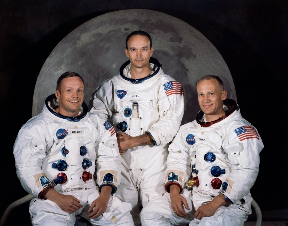

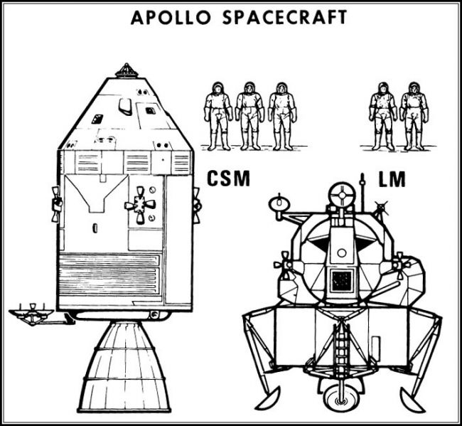
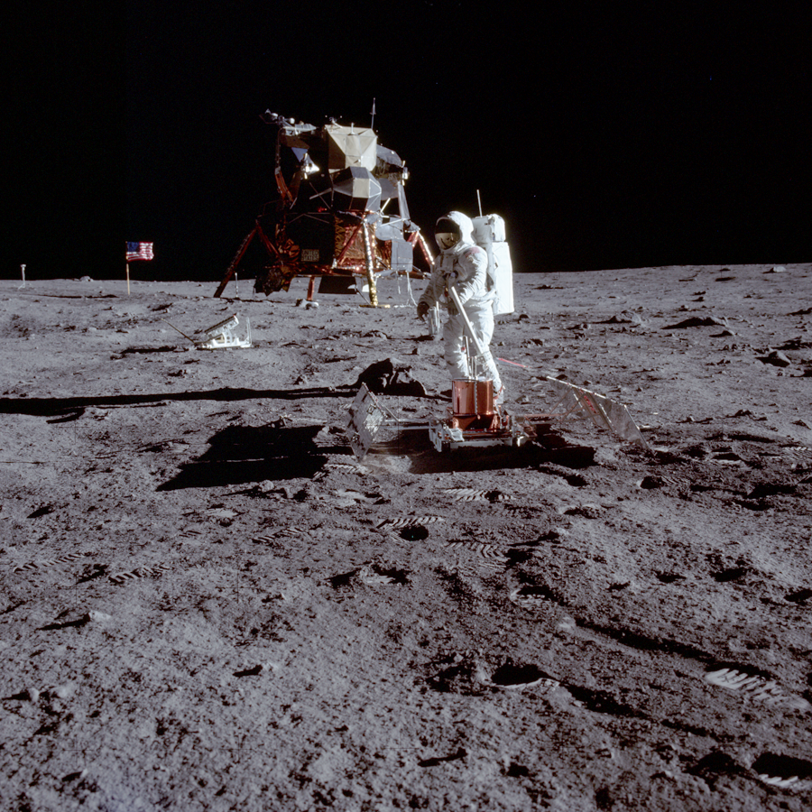
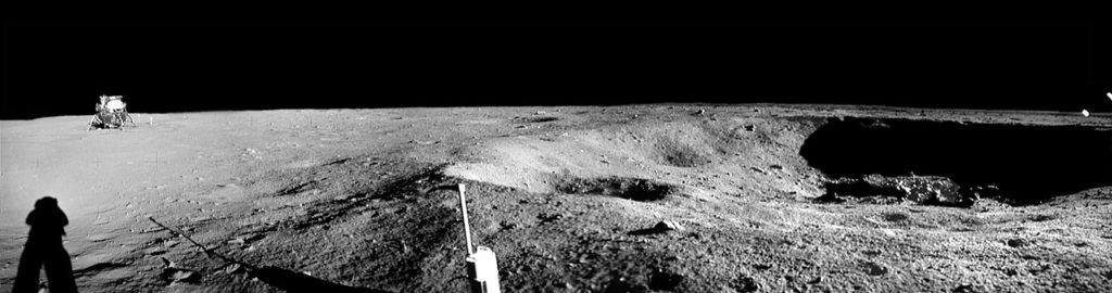
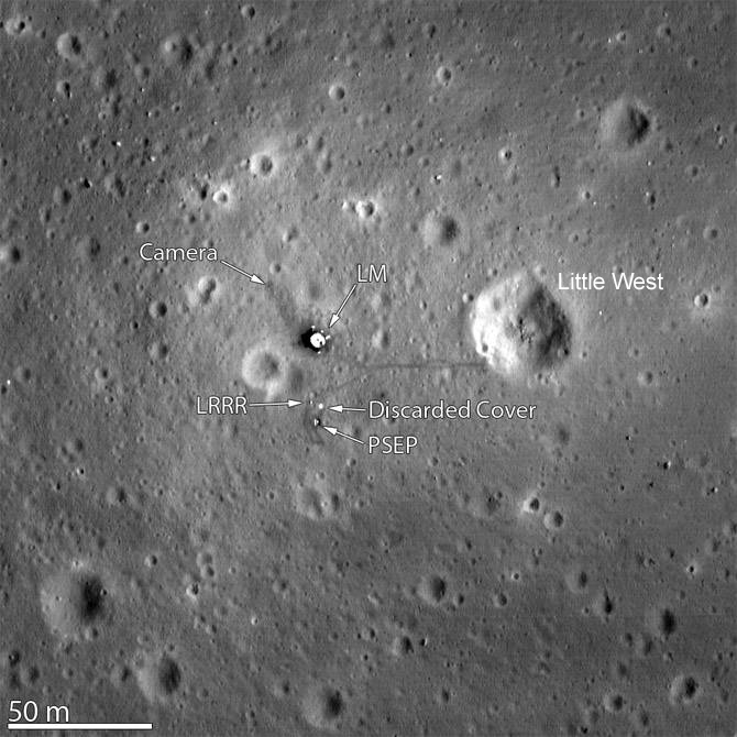
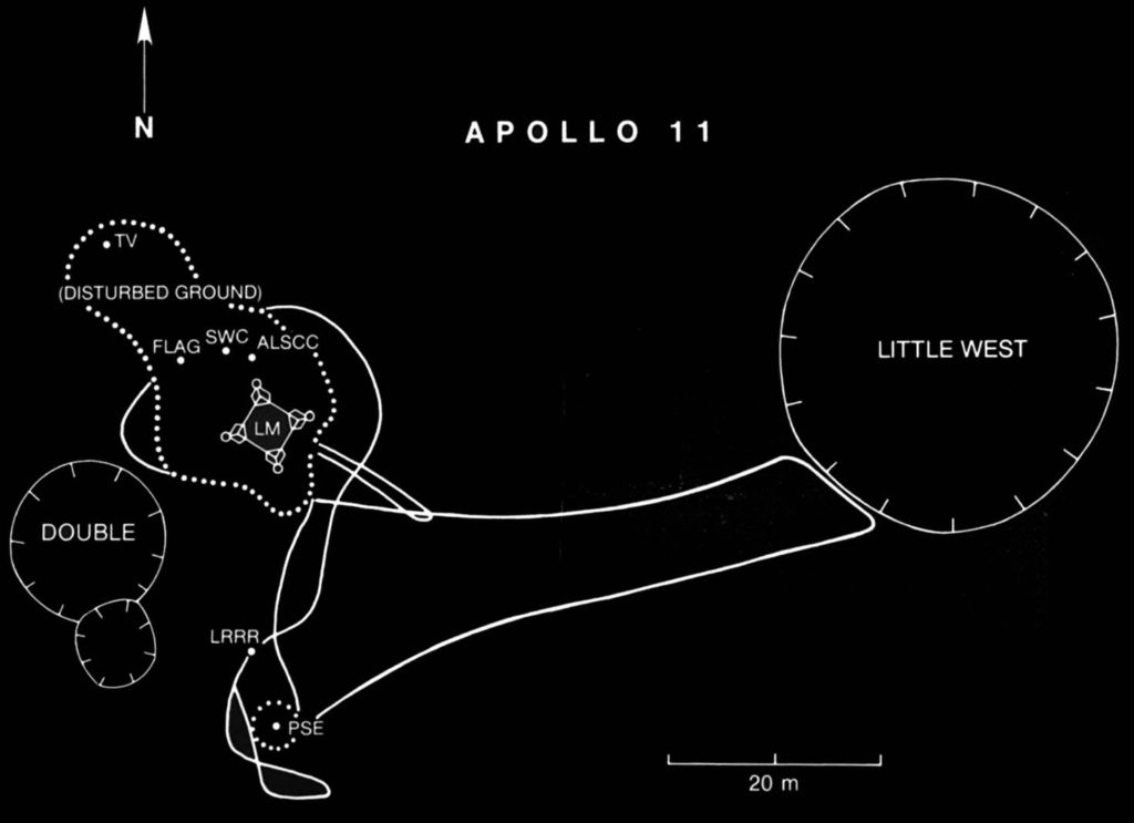
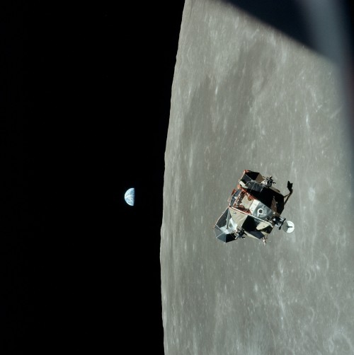

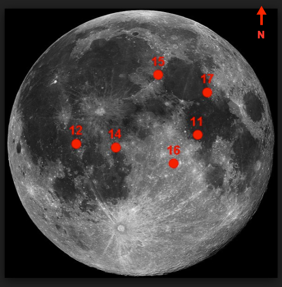
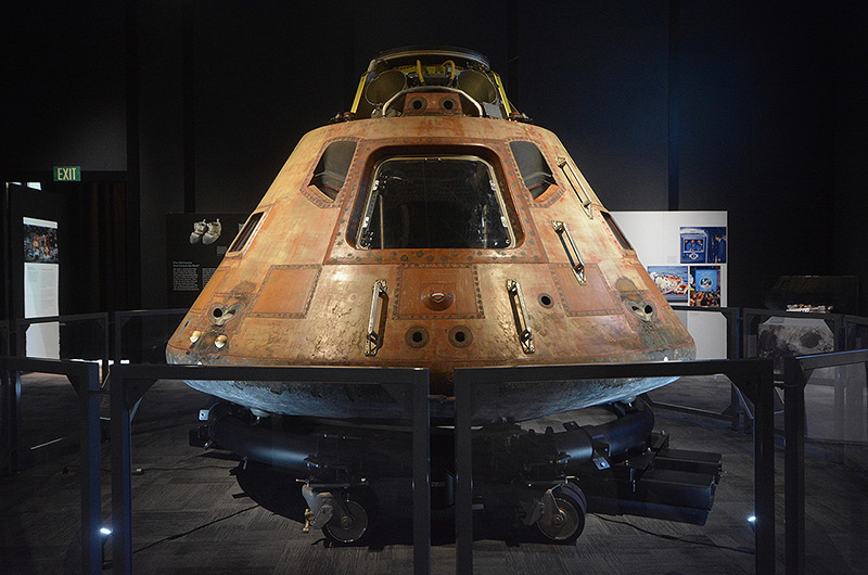
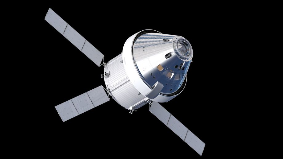
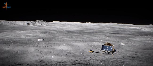
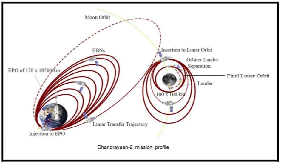
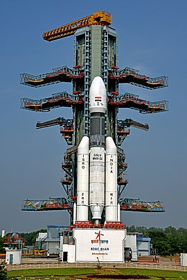
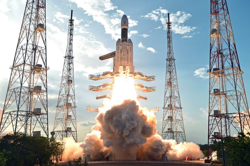
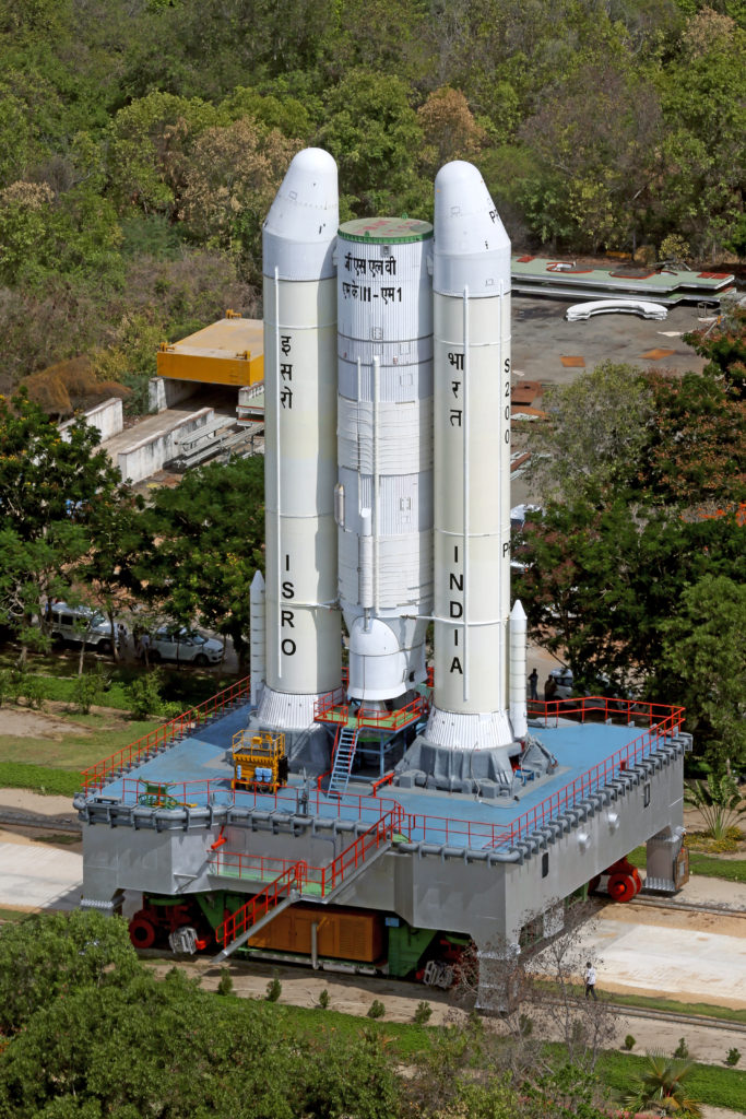
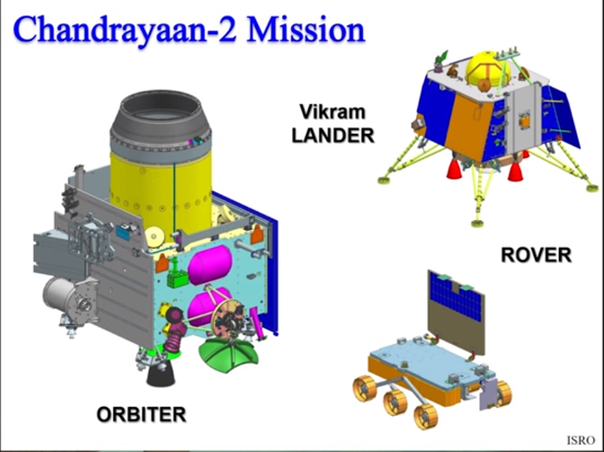
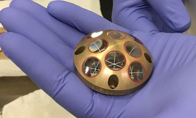
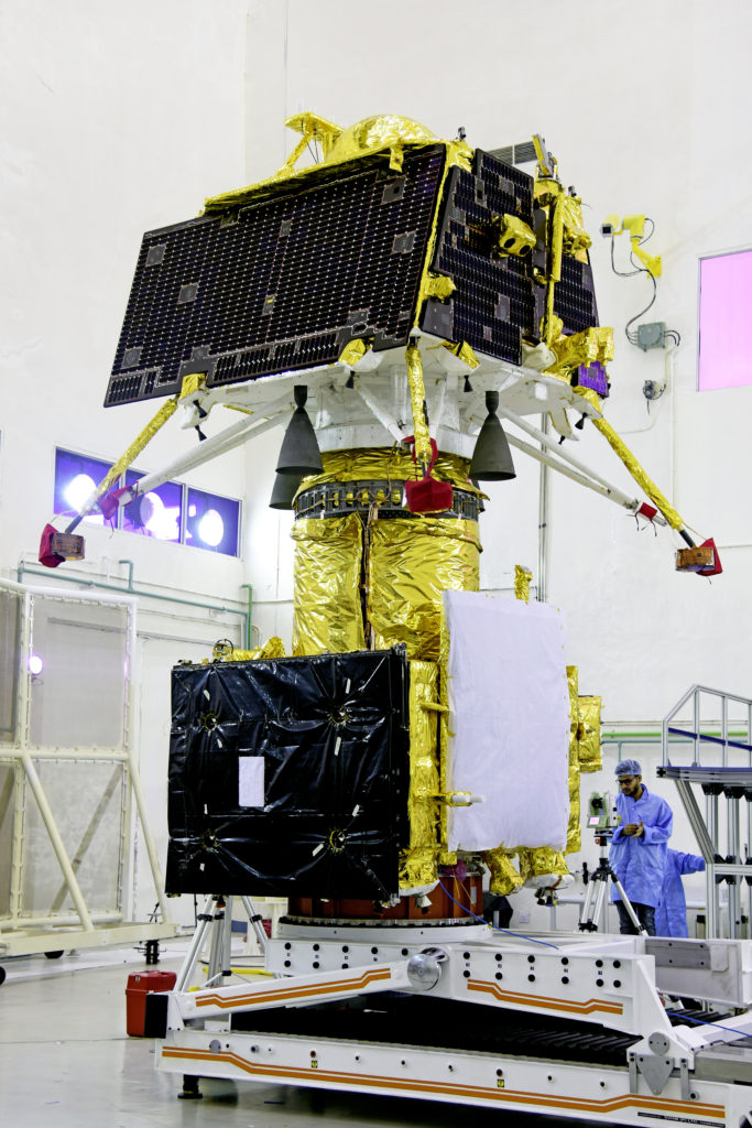
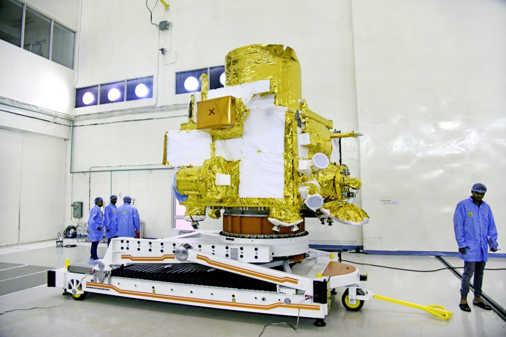
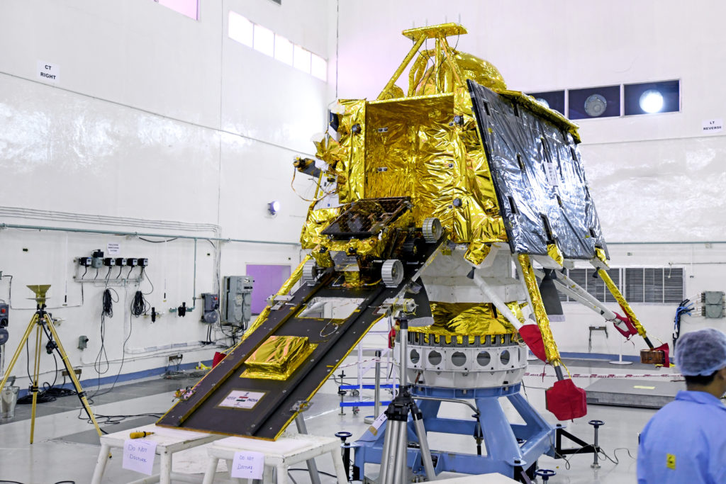
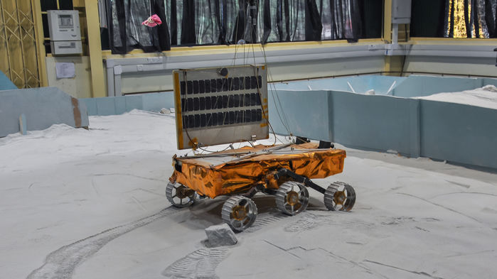
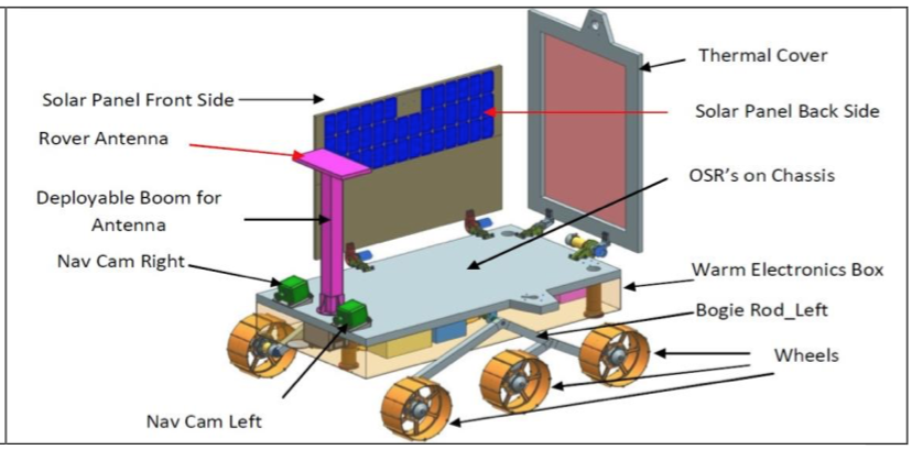
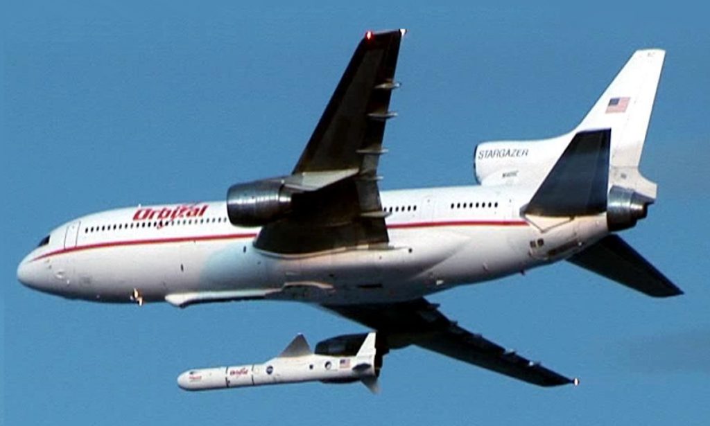
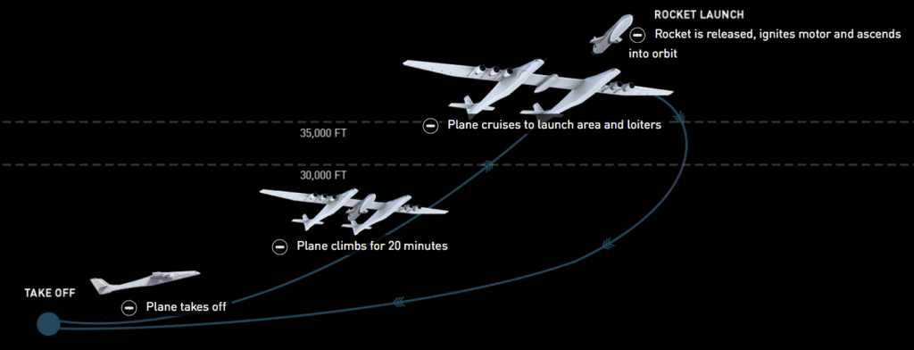
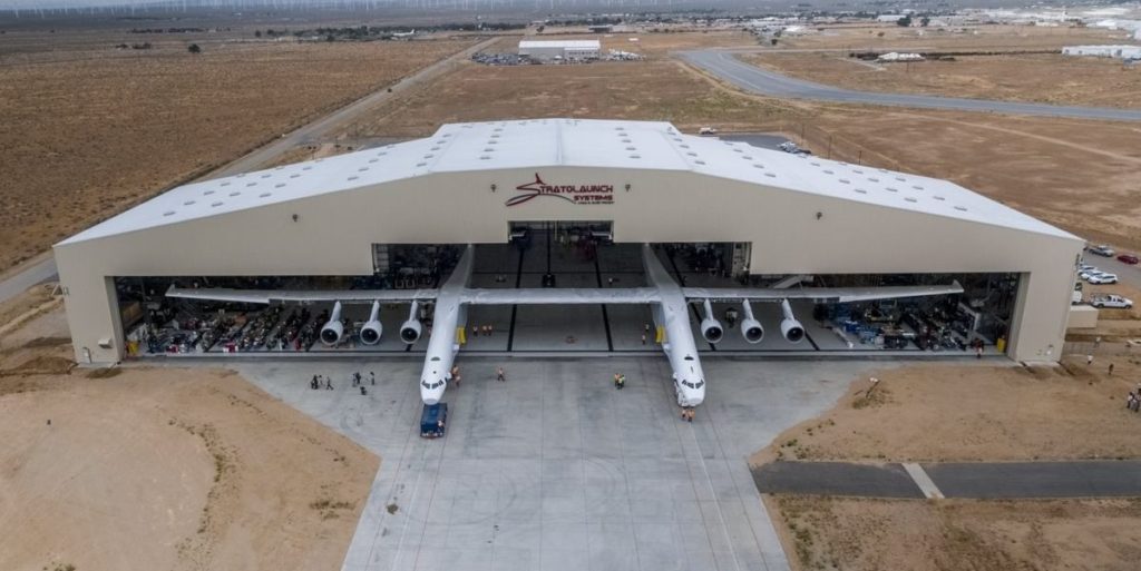
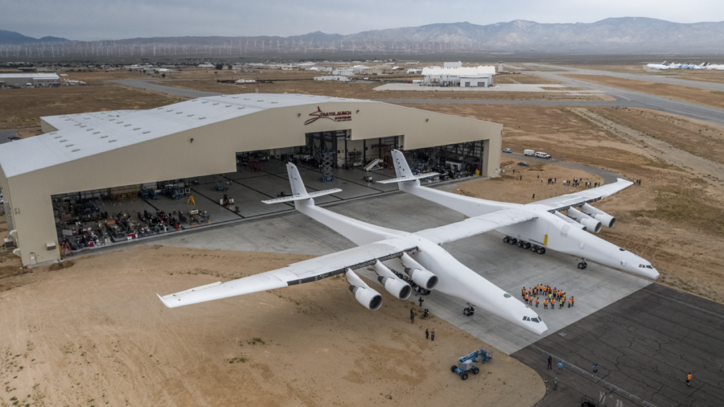
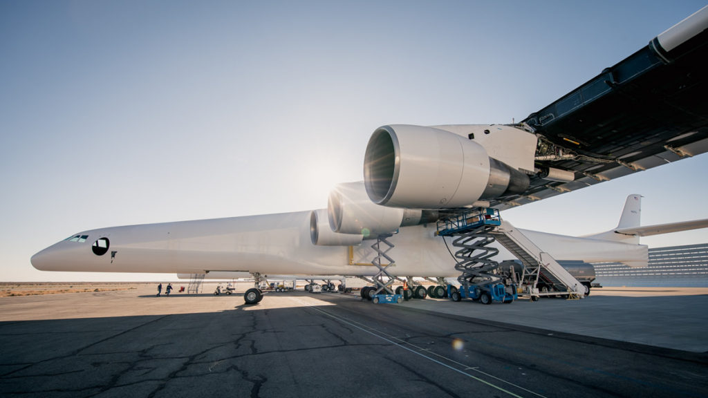
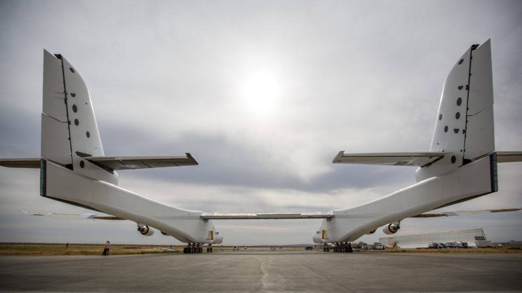
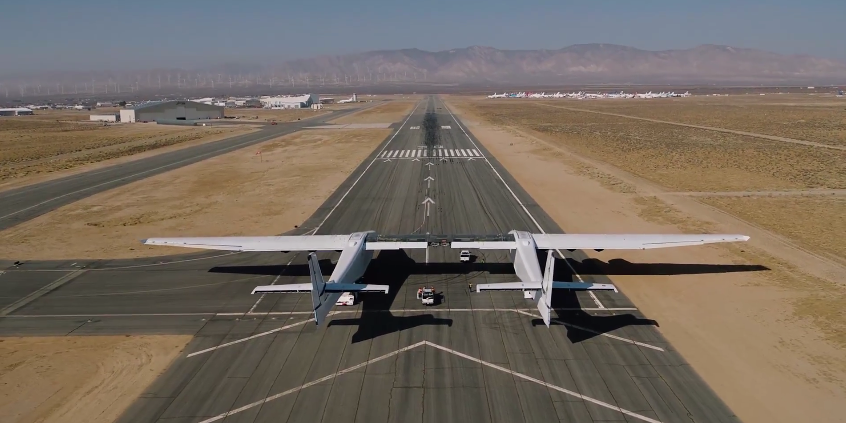
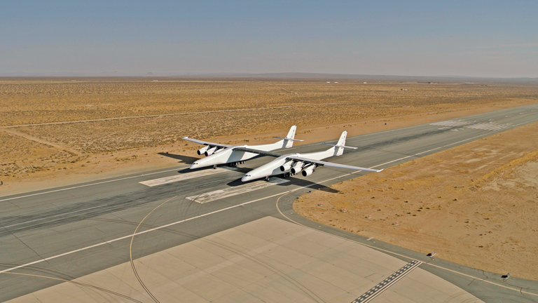
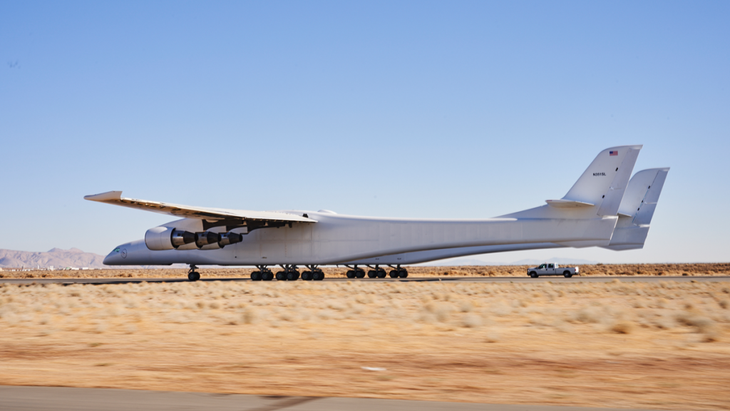
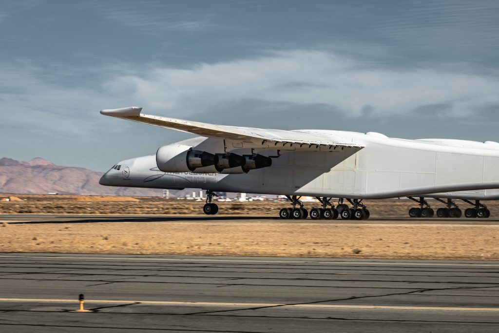

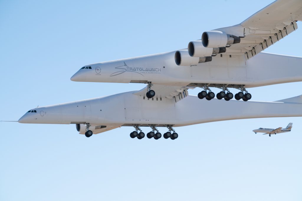
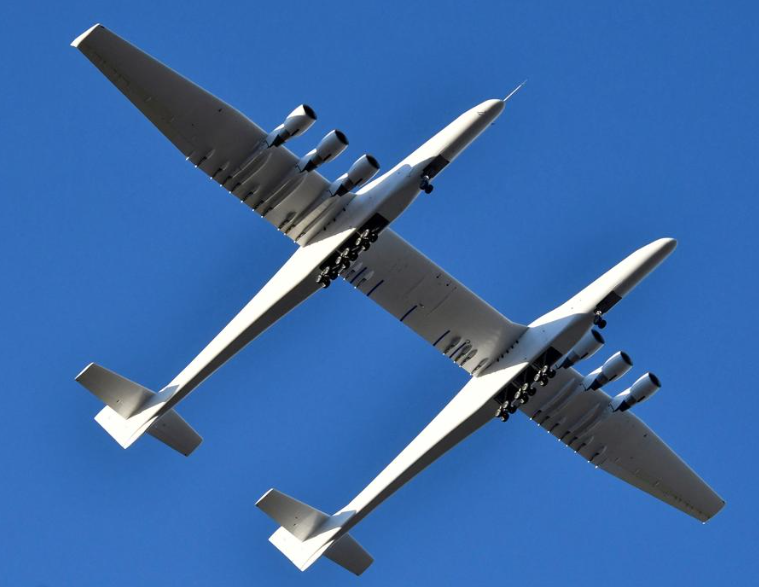
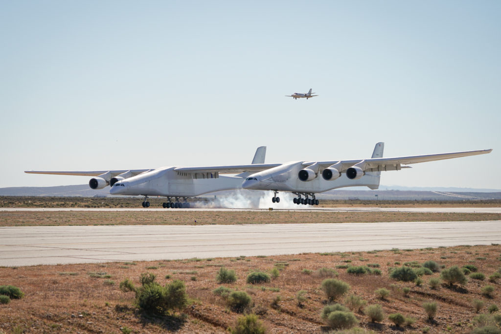

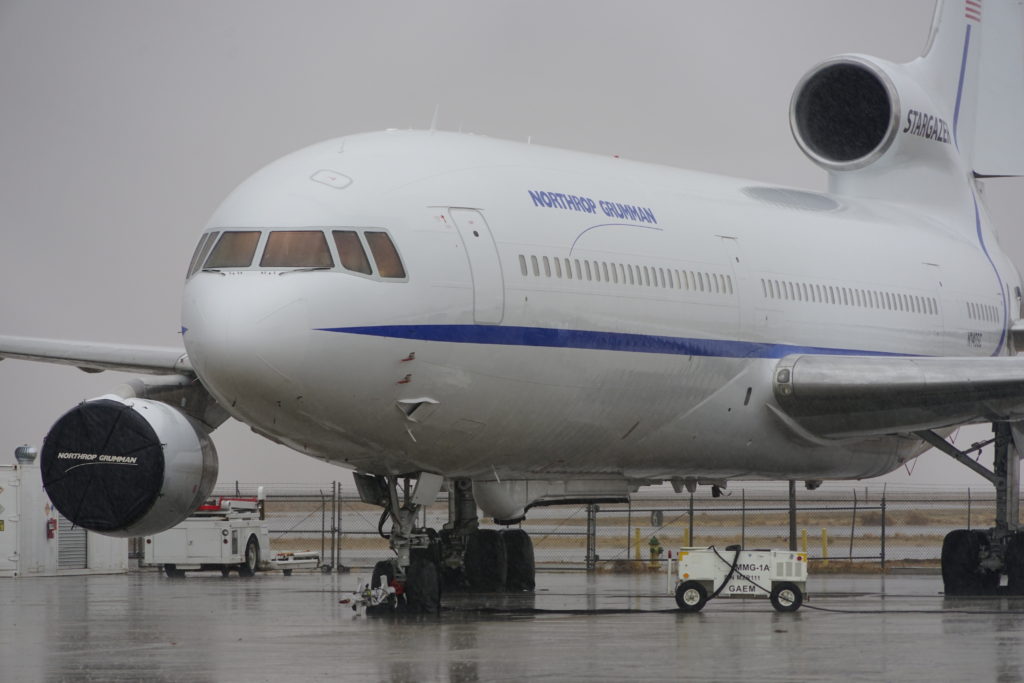
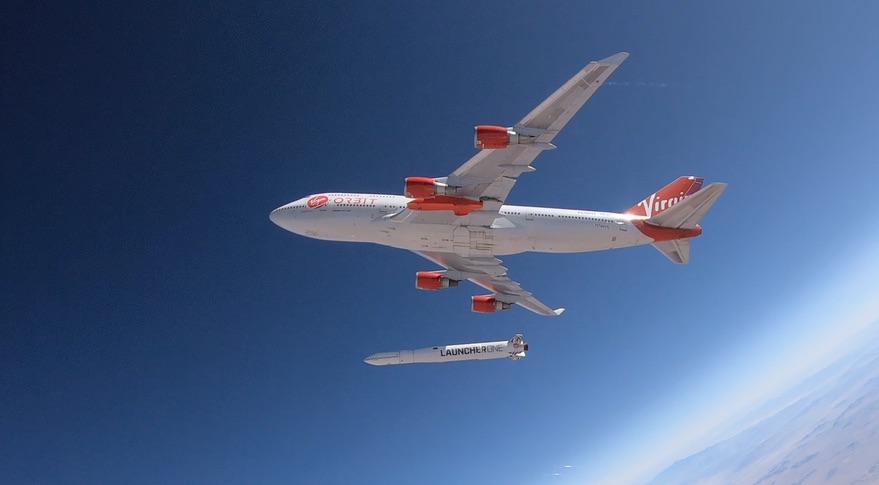
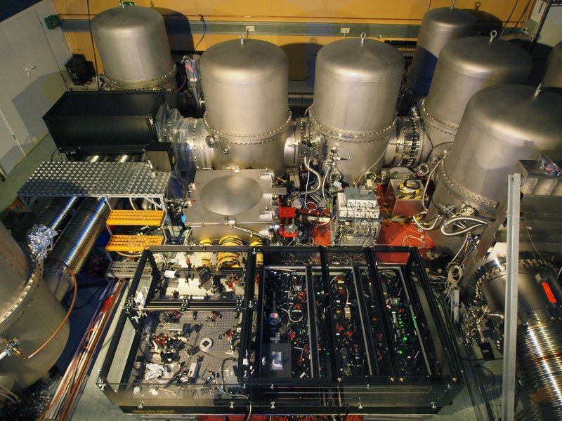
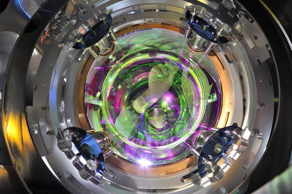
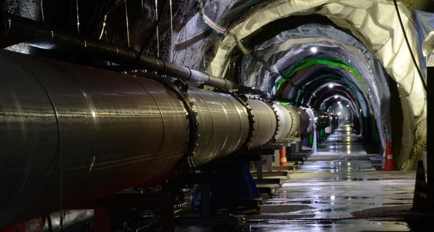
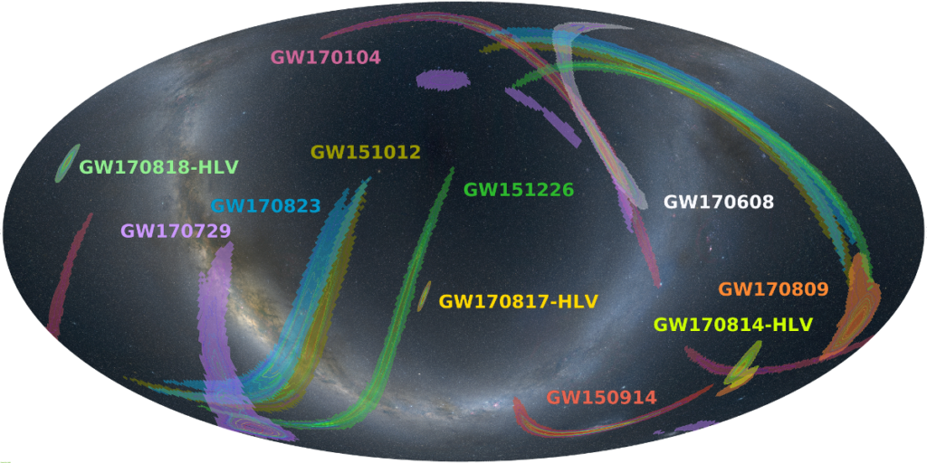
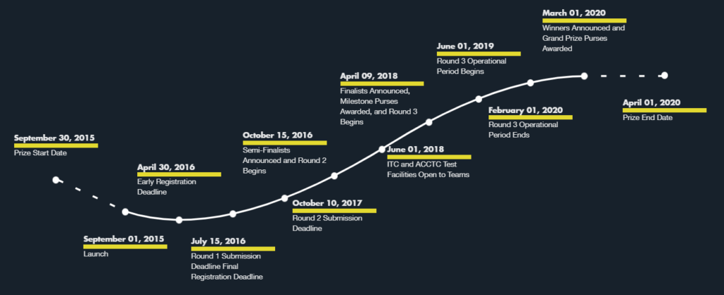
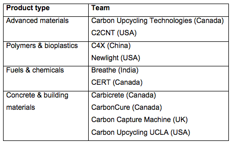
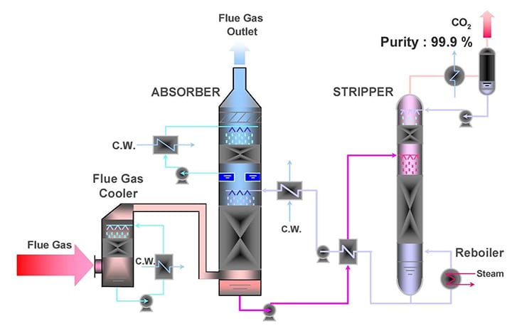
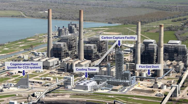
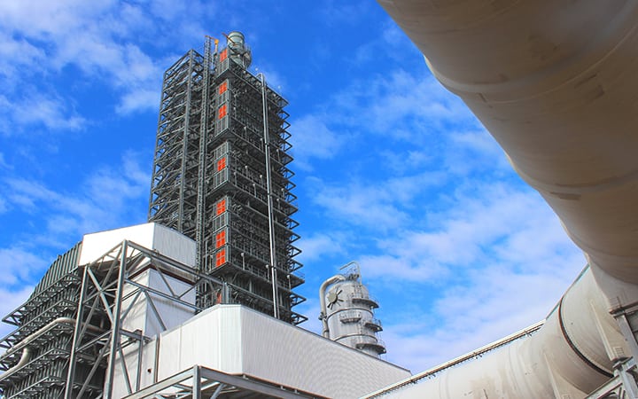
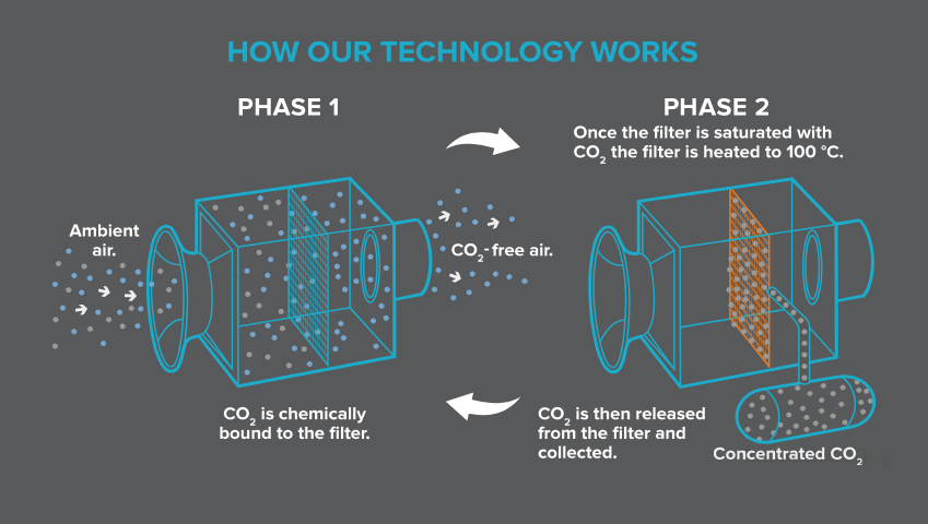
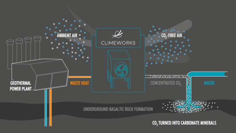


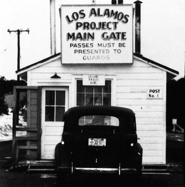
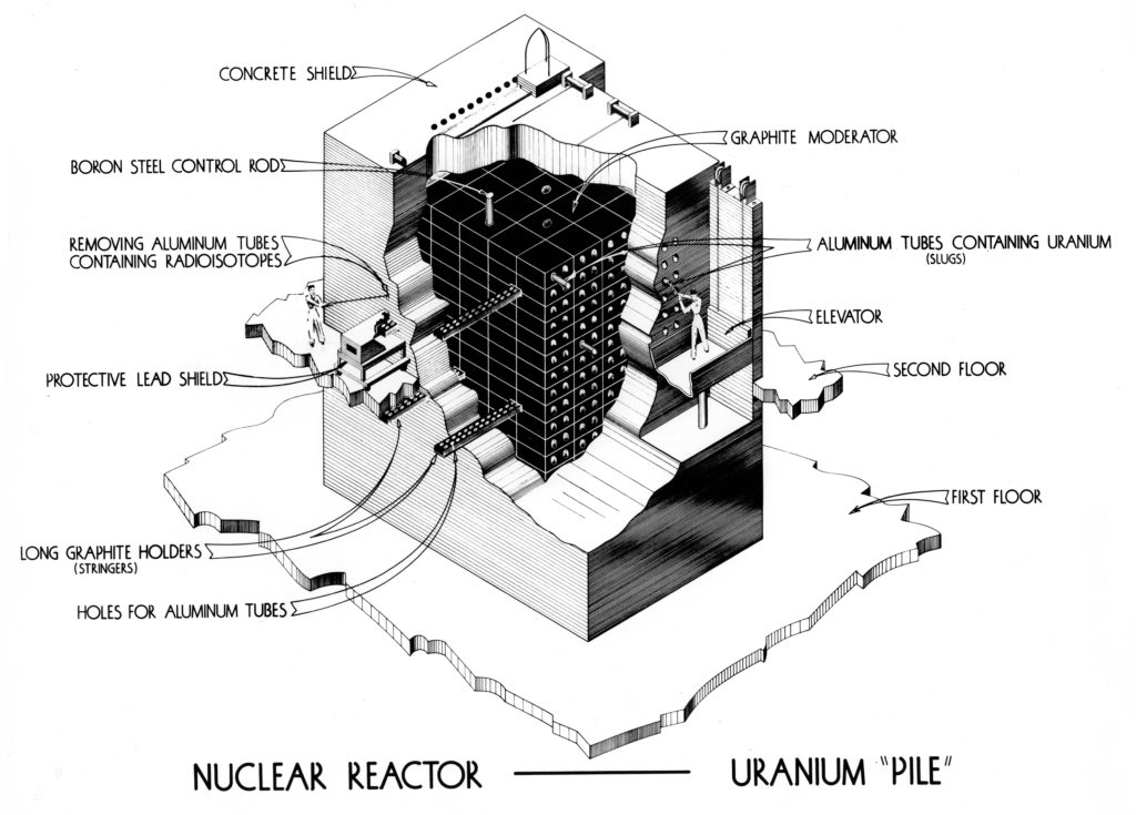
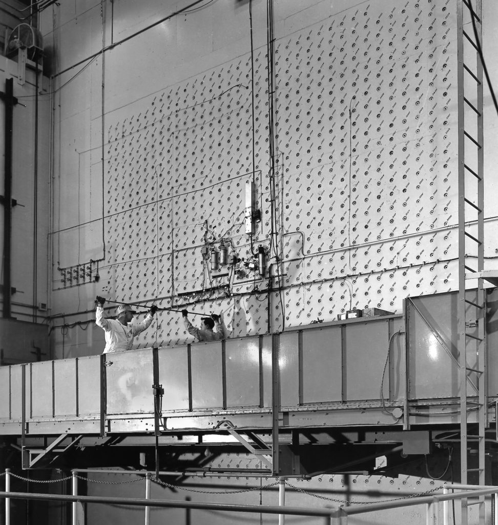
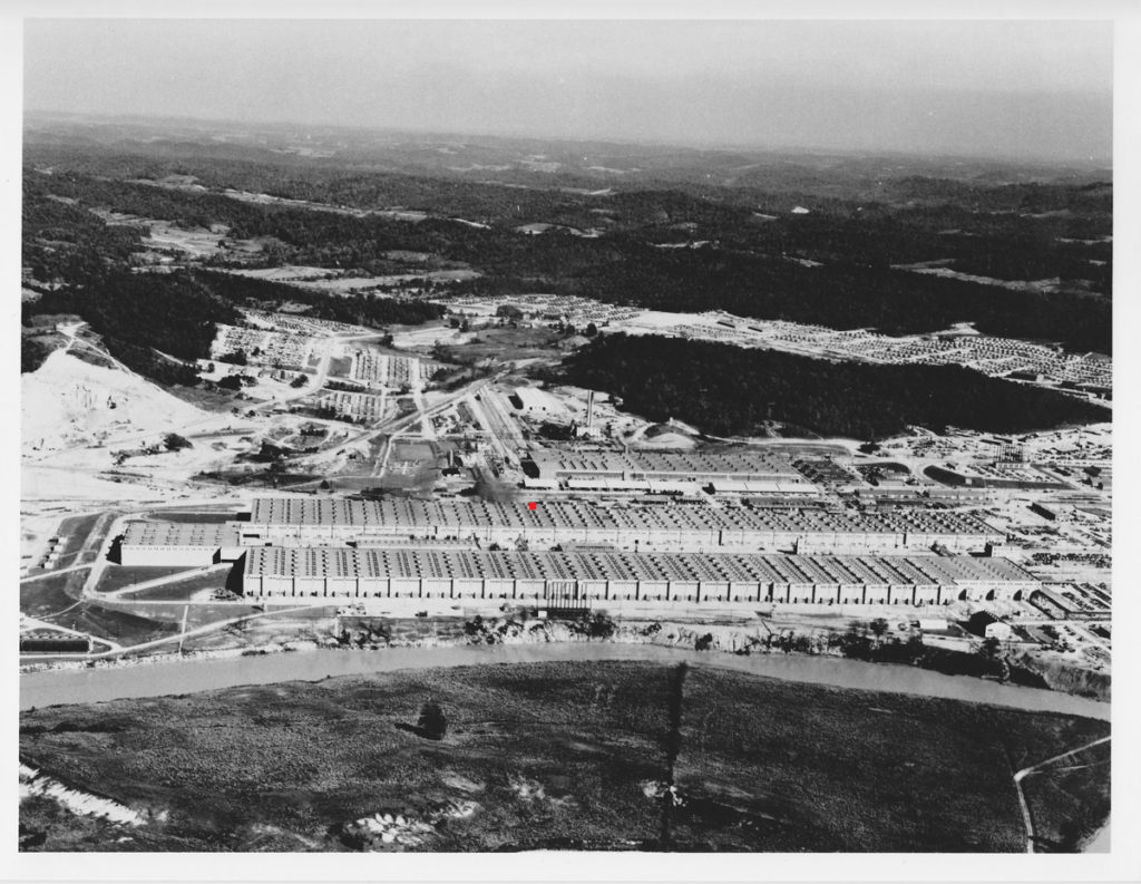
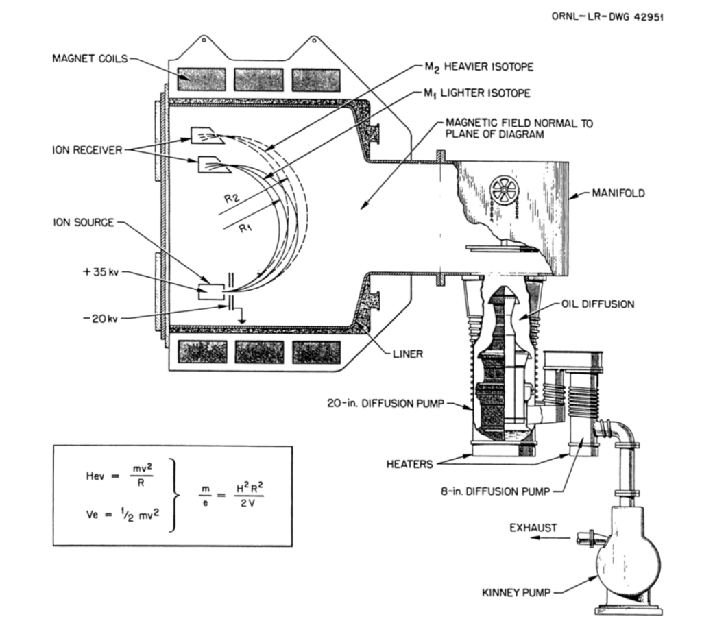
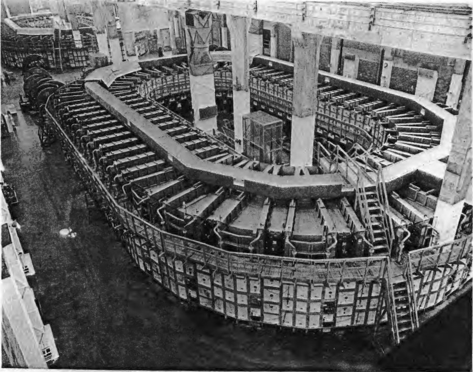
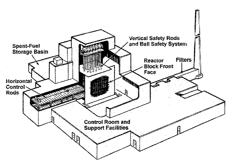
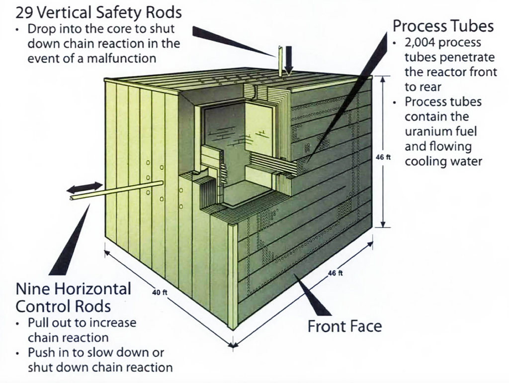
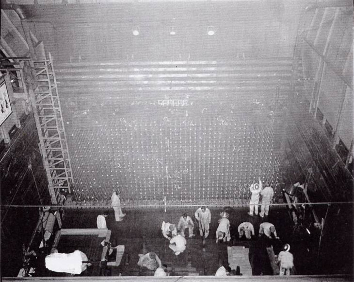
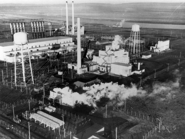
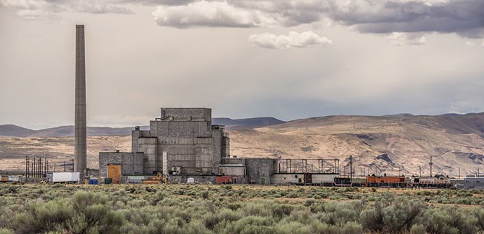
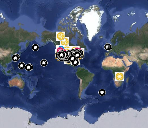
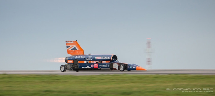

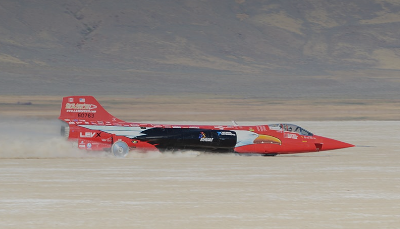
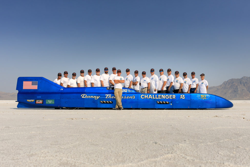
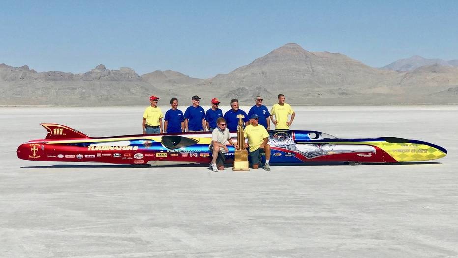
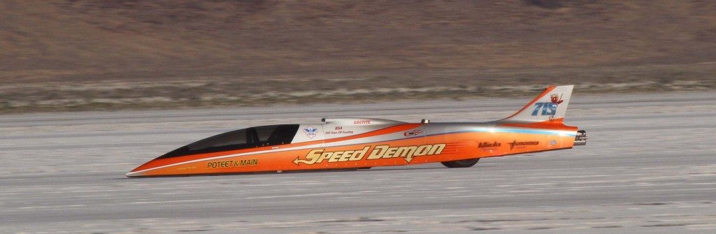
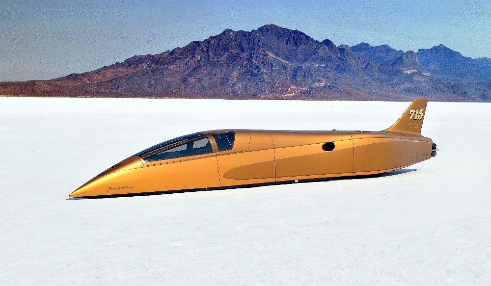
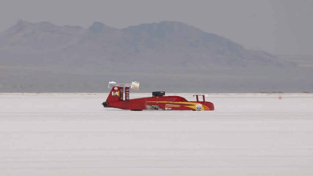
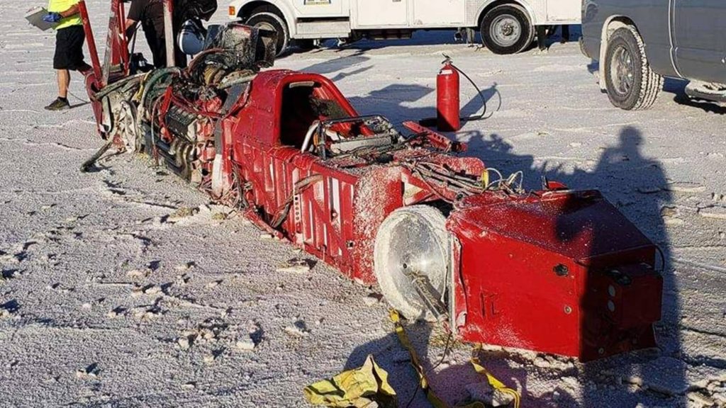
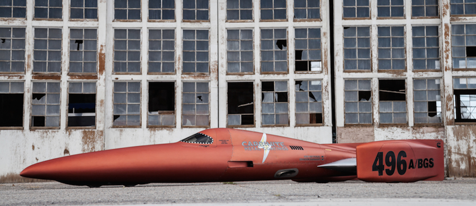
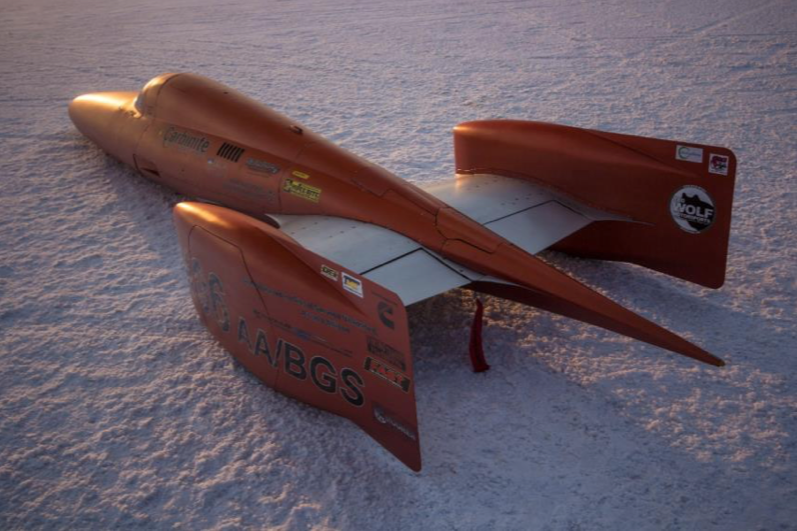
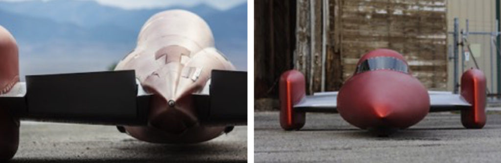
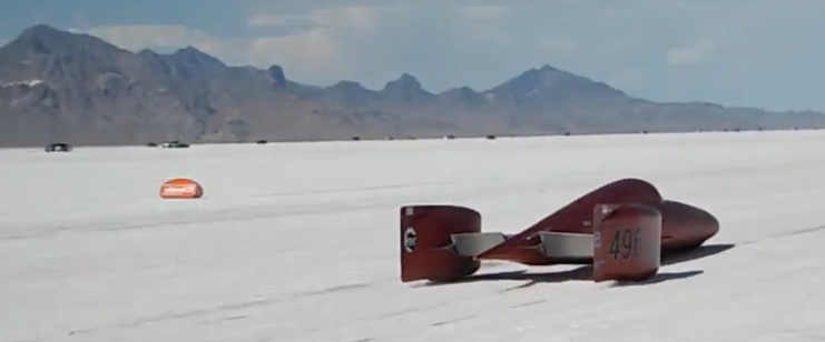
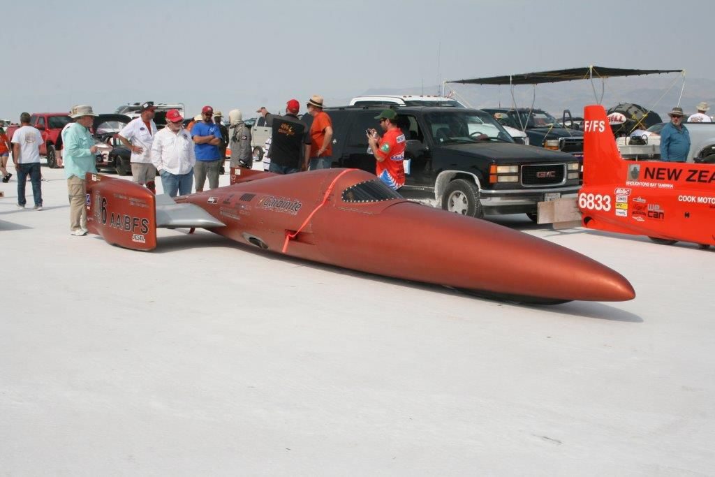
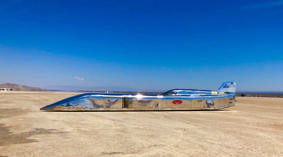
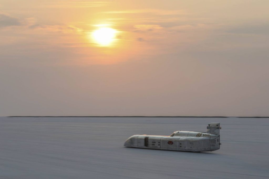
 Source:
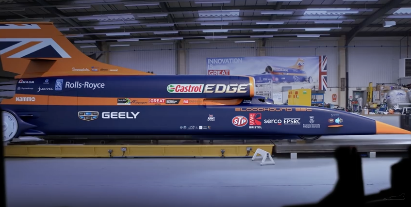
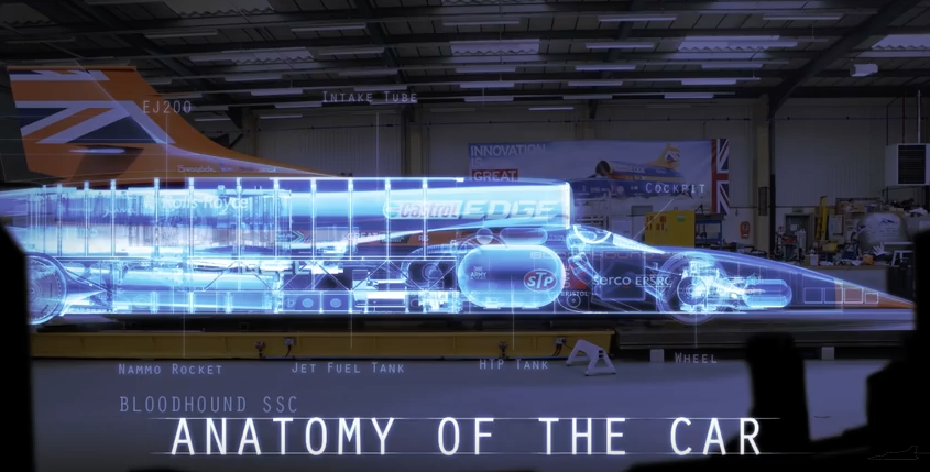


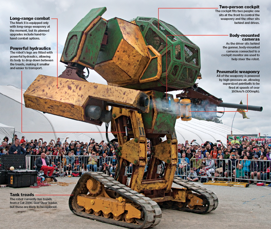


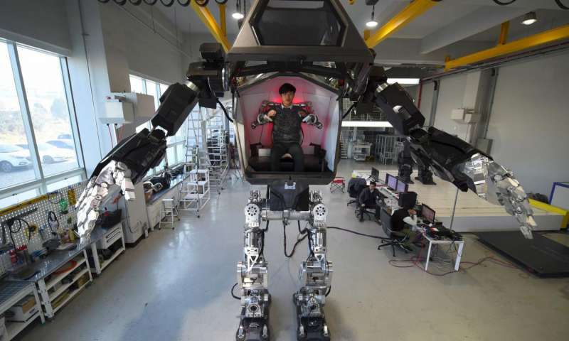
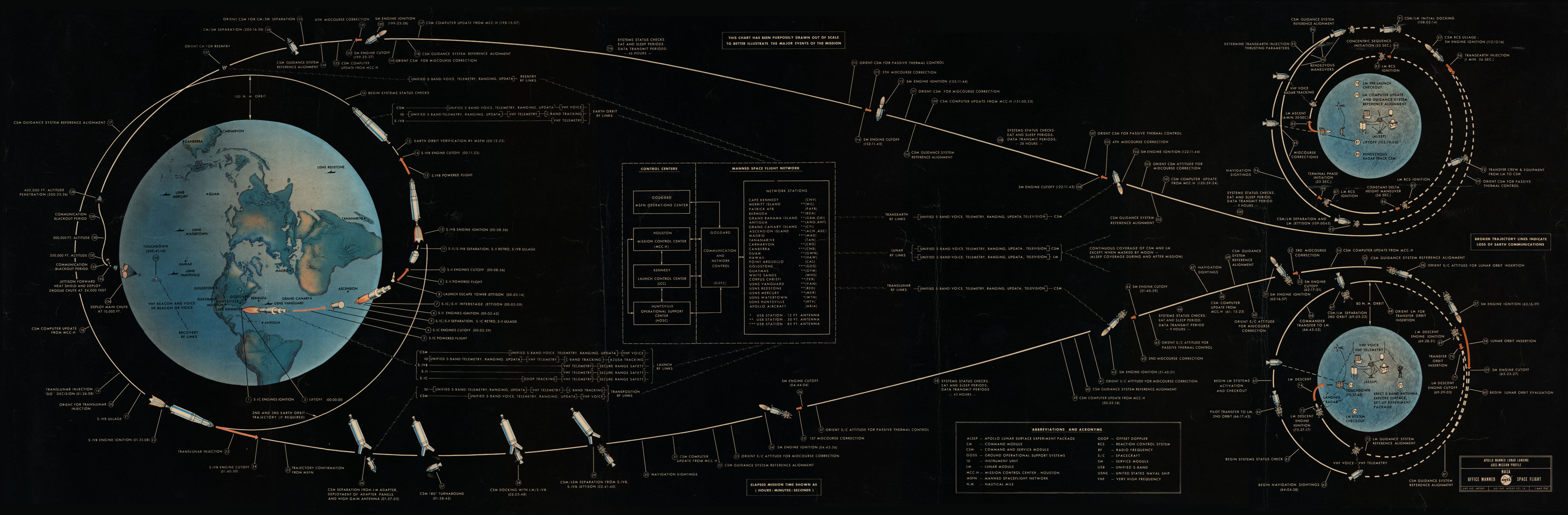