Peter Lobner, Updated 24 August 2021
From space, Antarctica gives the appearance of a large, ice-covered continental land mass surrounded by the Southern Ocean. The satellite photo mosaic, below, reinforces that illusion. Very little ice-free rock is visible, and it’s hard to distinguish between the continental ice sheet and ice shelves that extend into the sea.
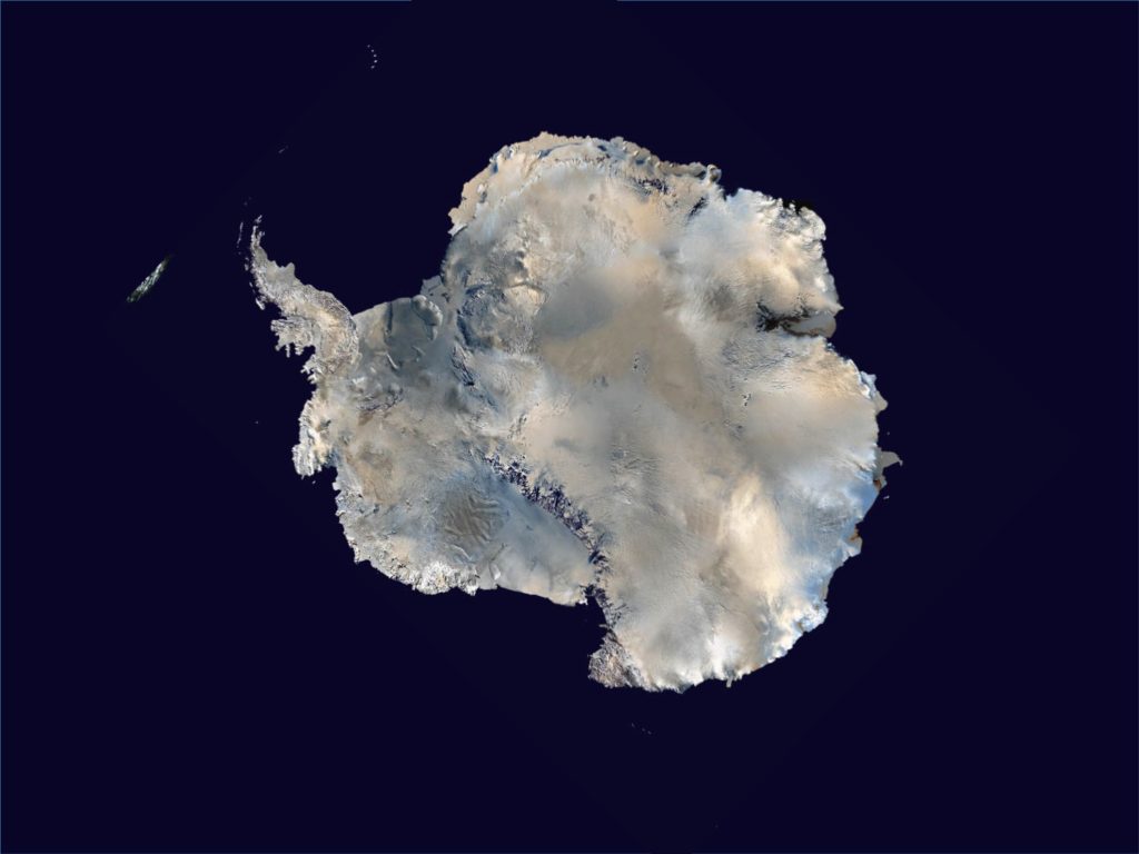
adapted to the same orientation as the following maps.
Source. https://geology.com/world/antarctica-satellite-image.shtml
The following topographical map presents the surface of Antarctica in more detail, and shows the many ice shelves (in grey) that extend beyond the actual coastline and into the sea. The surface contour lines on the map are at 500 meter (1,640 ft) intervals.
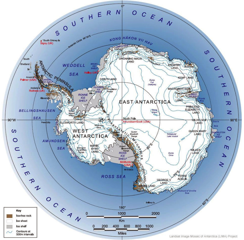
Source: LIMA Project (Landsat Image Mosaic of Antarctica) via Wikipedia
The highest elevation of the ice sheet is 4,093 m (13,428 ft) at Dome Argus (aka Dome A), which is located in the East Antarctic Ice Sheet, about 1,200 kilometers (746 miles) inland. The highest land elevation in Antarctica is Mount Vinson, which reaches 4,892 meters (16,050 ft) on the north part of a larger mountain range known as Vinson Massif, near the base of the Antarctic Peninsula. This topographical map does not provide information on the continental bed that underlies the massive ice sheets.
A look at the bedrock under the ice sheets: Bedmap2 and BedMachine
In 2001, the British Antarctic Survey (BAS) released a topographical map of the bedrock that underlies the Antarctic ice sheets and the coastal seabed derived from data collected by international consortia of scientists since the 1950s. The resulting dataset was called BEDMAP1.
In a 2013 paper, P. Fretwell, et al. (a very big team of co-authors), published the paper, “Bedmap2: Improved ice bed, surface and thickness datasets for Antarctica,” which included the following bed elevation map, with bed elevations color coded as indicated in the scale on the left. As you can see, large portions of the Antarctic “continental” bedrock are below sea level.
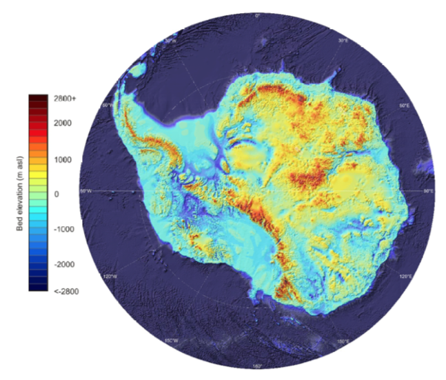
You can read the 2013 Fretwell paper here: https://www.the-cryosphere.net/7/375/2013/tc-7-375-2013.pdf
For an introduction to Antarctic ice sheet thickness, ice flows, and the topography of the underlying bedrock, please watch the following short (1:51) 2013 video, “Antarctic Bedrock,” by the National Aeronautics and Space Administration’s (NASA’s) Scientific Visualization Studio:
NASA explained:
- “In 2013, BAS released an update of the topographic dataset called BEDMAP2 that incorporates twenty-five million measurements taken over the past two decades from the ground, air and space.”
- “The topography of the bedrock under the Antarctic Ice Sheet is critical to understanding the dynamic motion of the ice sheet, its thickness and its influence on the surrounding ocean and global climate. This visualization compares the new BEDMAP2 dataset, released in 2013, to the original BEDMAP1 dataset, released in 2001, showing the improvements in resolution and coverage. This visualization highlights the contribution that NASA’s mission Operation IceBridge made to this important dataset.”
On 12 December 2019, a University of California Irvine (UCI)-led team of glaciologists unveiled the most accurate portrait yet of the contours of the land beneath Antarctica’s ice sheet. The new topographic map, named “BedMachine Antarctica,” is shown below.
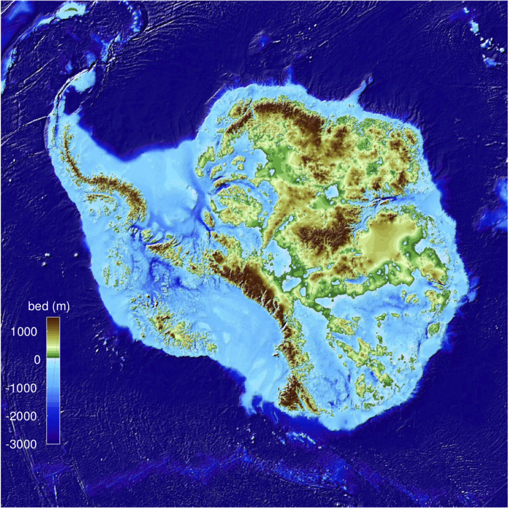
Credit: Mathieu Morlighem / UCI
UCI reported:
- “The new Antarctic bed topography product was constructed using ice thickness data from 19 different research institutes dating back to 1967, encompassing nearly a million line-miles of radar soundings. In addition, BedMachine’s creators utilized ice shelf bathymetry measurements from NASA’s Operation IceBridge campaigns, as well as ice flow velocity and seismic information, where available. Some of this same data has been employed in other topography mapping projects, yielding similar results when viewed broadly.”
- “By basing its results on ice surface velocity in addition to ice thickness data from radar soundings, BedMachine is able to present a more accurate, high-resolution depiction of the bed topography. This methodology has been successfully employed in Greenland in recent years, transforming cryosphere researchers’ understanding of ice dynamics, ocean circulation and the mechanisms of glacier retreat.”
- “BedMachine relies on the fundamental physics-based method of mass conservation to discern what lies between the radar sounding lines, utilizing highly detailed information on ice flow motion that dictates how ice moves around the varied contours of the bed.”
The net result is a much higher resolution topographical map of the bedrock that underlies the Antarctic ice sheets. The authors note:“This transformative description of bed topography redefines the high- and lower-risk sectors for rapid sea level rise from Antarctica; it will also significantly impact model projections of sea level rise from Antarctica in the coming centuries.”
You can take a visual tour of BedMachine’s high-precision model of Antarctic’s ice bed topography here. Enjoy your trip.
There is significant geothermal heating under parts of Antarctica’s bedrock
West Antarctica and the Antarctic Peninsula form a connected rift / fault zone that includes about 60 active and semi-active volcanoes, which are shown as red dots in the following map.
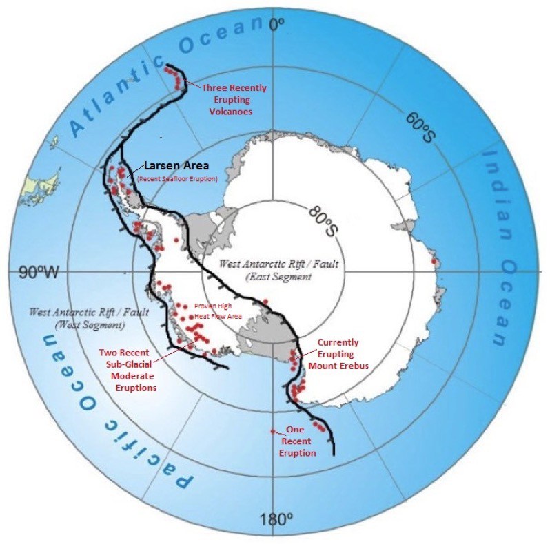
Source: James Kamis, Plate Climatology, 4 July 2017
In a 29 June 2018 article on the Plate Climatology website, author James Kamis presents evidence that the fault / rift system underlying West Antarctica generates a significant geothermal heat flow into the bedrock and is the source of volcanic eruptions and sub-glacial volcanic activity in the region. The heat flow into the bedrock and the observed volcanic activity both contribute to the glacial melting observed in the region. You can read this article here:
http://www.plateclimatology.com/geologic-forces-fueling-west-antarcticas-larsen-ice-shelf-cracks/
The correlation between the locations of the West Antarctic volcanoes and the regions of higher heat flux within the fault / rift system are evident in the following map, which was developed in 2017 by a multi-national team.
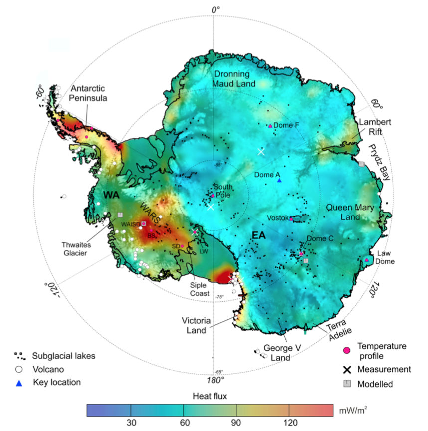
The authors note: “Direct observations of heat flux are difficult to obtain in Antarctica, and until now continent-wide heat flux maps have only been derived from low-resolution satellite magnetic and seismological data. We present a high-resolution heat flux map and associated uncertainty derived from spectral analysis of the most advanced continental compilation of airborne magnetic data. …. Our high-resolution heat flux map and its uncertainty distribution provide an important new boundary condition to be used in studies on future subglacial hydrology, ice sheet dynamics, and sea level change.” This Geophysical Research Letter is available here:
https://agupubs.onlinelibrary.wiley.com/doi/pdf/10.1002/2017GL075609
The results of six Antarctic heat flux models developed from 2004 to 2017 were compared by Brice Van Liefferinge in his 2018 PhD thesis. His results, shown below, are presented on the Cryosphere Sciences website of the European Sciences Union (EGU).
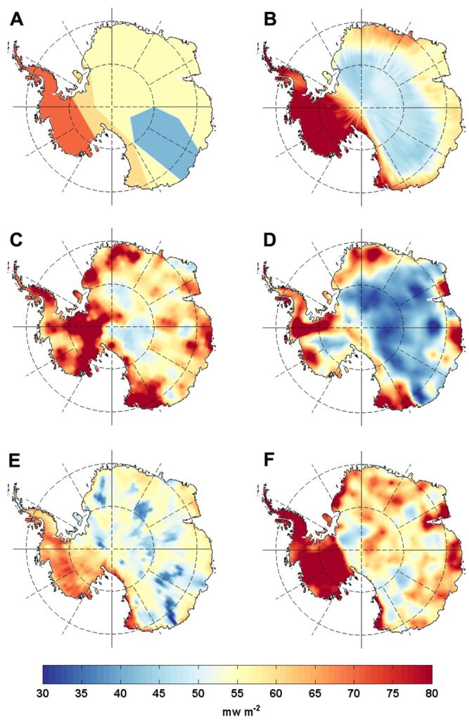
Regarding his comparison of Antarctic heat flux models, Van Liefferinge reported:
- “As a result, we know that the geology determines the magnitude of the geothermal heat flux and the geology is not homogeneous underneath the Antarctic Ice Sheet: West Antarctica and East Antarctica are significantly distinct in their crustal rock formation processes and ages.”
- “To sum up, although all geothermal heat flux data sets agree on continent scales (with higher values under the West Antarctic ice sheet and lower values under East Antarctica), there is a lot of variability in the predicted geothermal heat flux from one data set to the next on smaller scales. A lot of work remains to be done …”
The effects of geothermal heating are particularly noticeable at Deception Island, which is part of a collapsed and still active volcanic crater near the tip of the Antarctic Peninsula. This high heat flow volcano is in the same major fault zone as the rapidly melting / breaking-up Larsen Ice Shelf. The following map shows the faults and volcanoes in this region.
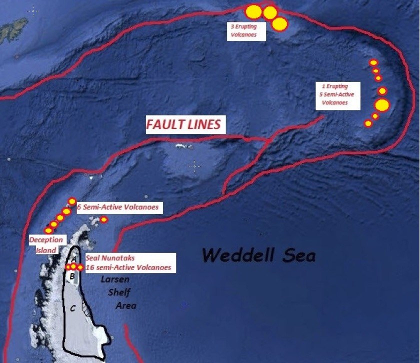
Source: James Kamis, Plate Climatology, 4 July 2017
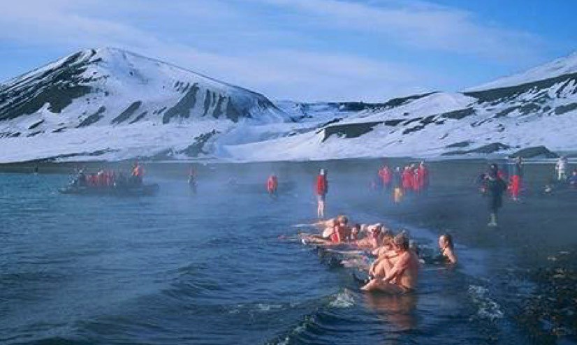
Source: Public domain
So, if you take a cruise to Antarctica and the Cruise Director offers a “polar bear” plunge, I suggest that you wait until the ship arrives at Deception Island. Remember, this warm water is not due to climate change. You’re in a volcano.
For more information on Bedmap 2 and BedMachine:
- P. Fretwell, et al., “Bedmap2: Improved ice bed, surface and thickness datasets for Antarctica,” Cryosphere, 7, 375–393 (2013): https://www.the-cryosphere.net/7/375/2013/tc-7-375-2013.pdf
- “Antarctic Bedrock,” Visualizations by Cindy Starr, NASA Scientific Visualization Studio, Released on June 4, 2013: https://svs.gsfc.nasa.gov/4060
- “Team releases high-precision map of Antarctic ice sheet bed topography, “ University of California Irvine, 12 December 2019: https://phys.org/news/2019-12-team-high-precision-antarctic-ice-sheet.html
- Morlighem, M., Rignot, E., Binder, T. et al. “Deep glacial troughs and stabilizing ridges unveiled beneath the margins of the Antarctic ice sheet,” Nature Geoscience (2019) doi:10.1038/s41561-019-0510-8: https://www.nature.com/articles/s41561-019-0510-8
- Jessica Merzforf, “NASA’s Operation IceBridge completes 11 years of polar surveys,” NASA Goddard Space Flight Center, 12 December 2019: https://phys.org/news/2019-12-nasa-icebridge-years-polar-surveys.html
- “Antarctic ice sheets could be at greater risk of melting than previously thought,” University of South Australia, 2 December 2019: https://phys.org/news/2019-12-antarctic-ice-sheets-greater-previously.html
More information on geothermal heating in the West Antarctic rift / fault zone:
- James Kamis, “Three New Studies Confirm Volcanism Is Melting West Antarctic Glaciers, Not Global Warming,” Plate Climatology, 29 June 2018: http://www.plateclimatology.com/three-new-studies-confirm-volcanism-is-melting-west-antarctic-glaciers-not-global-warming
- James Kamis, “Geologic Forces Fueling West Antarctica’s Larsen Ice Shelf Cracks,” Plate Climatology, 4 July 2017: http://www.plateclimatology.com/geologic-forces-fueling-west-antarcticas-larsen-ice-shelf-cracks/
- Yasmina M. Martos, et al., “Heat Flux Distribution of Antarctica Unveiled,” Geophysical Research Letters, Research Letter 10.1002/2017GL075609, published 30 November 2017: https://agupubs.onlinelibrary.wiley.com/doi/pdf/10.1002/2017GL075609
- Brice Van Liefferinge, “Geothermal heat flux in Antarctica: do we really know anything?” Cryosphere Sciences, 23 March 2018: https://blogs.egu.eu/divisions/cr/2018/03/23/image-of-the-week-geothermal-heat-flux-in-antarctica-do-we-really-know-anything/
- T. A. Jordan, et al., “Anomalously high geothermal flux near the South Pole,” Scientific Reports 8, Article 16785, 14 November 2018: https://www.nature.com/articles/s41598-018-35182-0
- Brandon Specktor, “Antarctica’s ‘Doomsday Glacier’ is fighting an invisible battle against the inner Earth, new study finds,” Live Science, 20 August 2021: https://www.livescience.com/antarctica-doomsday-glacier-geothermal-heat-map