Category Archives: Planetary science

NASA’s DART spacecraft impact measurably redirected the asteroid Dimorphos

Peter Lobner, updated 28 July 2023

NASA’s Double Asteroid Redirection Test (DART), which was launched on 24 November 2021, was the first test of a technology for defending Earth against potential asteroid or comet hazards. DART’s target was the small “moonlet” named Dimorphos orbiting the larger near-Earth asteroid Didymos, which itself is only a half mile in diameter.  You can explore at the Didymos – Dimorphos binary system on NASA’s Solar System Exploration webpage here: https://solarsystem.nasa.gov/asteroids-comets-and-meteors/asteroids/didymos/in-depth/

Simulation of the Didymos – Dimorphos binary system. 
Source: NASA’s Solar System Exploration
Actual view of the Didymos – Dimorphos binary system as 
DART approached impact with Dimorphos (background). 
Source: NASA / JHAPL

The goal is for the DART spacecraft was to strike the moonlet Dimorphos at high speed while being trailed by another small spacecraft, the Italian Space Agency’s (ASI) cubesat, dubbed LICIACube, that would directly observe the encounter and report back to NASA and ASI. 

By comparing pre- and post-impact measurements made with powerful Earth-based and orbiting telescopes, the NASA / Johns Hopkins Applied Physics Lab (JHAPL) team could determine what changes occurred to Dimorphos’ orbit around Didymos. These results will help assess the feasibility of using a high-energy impactor as a tool for deflecting the trajectory of an asteroid, particularly one that represents a significant risk to Earth.  Learn more about the DART spacecraft and its mission objectives on NASA’s Planetary Defense Coordination Office website here: https://www.nasa.gov/planetarydefense/dart/dart-news

NASA successfully guided DART to a collision with Dimorphos on 26 September 2022.   You can watch the final five minutes of DART’s approach to the Didymos – Dimorphos binary system up to the final image before impact here: https://www.nasa.gov/feature/dart-s-final-images-prior-to-impact

DART closeup image of Dimorphos moments before impact.
Source: NASA / JHAPL
ASI’s LICIACube image just before its closest approach to Dimorphos (background). The debris plume cast off from Dimorphos after DART’s impact is clearly visible. Didymos is in the foreground. Source: ASI / NASA

The Hubble Space Telescope was used to capture images of the impact.  The NASA/ESA Hubble Space Telescope team reported:

“The Hubble movie starts at 1.3 hours before impact. The first post-impact snapshot is 20 minutes after the event. Debris flies away from the asteroid in straight lines, moving faster than four miles per hour (fast enough to escape the asteroid’s gravitational pull, so it does not fall back onto the asteroid). The ejecta forms a largely hollow cone with long, stringy filaments.

At about 17 hours after the impact the debris pattern entered a second stage. The dynamic interaction within the binary system started to distort the cone shape of the ejecta pattern. The most prominent structures are rotating, pinwheel-shaped features. The pinwheel is tied to the gravitational pull of the companion asteroid, Didymos. 

Hubble next captures the debris being swept back into a comet-like tail by the pressure of sunlight on the tiny dust particles. This stretches out into a debris train where the lightest particles travel the fastest and farthest from the asteroid. The mystery is compounded later when Hubble records the tail splitting in two for a few days.”

8 October 2022 photo by the Hubble Space Telescope shows Dimorphos with its debris tail. Source: NASA/ESA/STScI/Hubble

The results are in, and on 1 March 2023, the NASA / JHAPL team reported a much greater change to Dimorphos’ orbit than originally expected.

“…the investigation team, led by Cristina Thomas of Northern Arizona University, arrived at two consistent measurements of the period change from the kinetic impact: 33 minutes, plus or minus one minute. This large change indicates the recoil from material excavated from the asteroid and ejected into space by the impact (known as ejecta) contributed significant momentum change to the asteroid, beyond that of the DART spacecraft itself.”

Source: NASA/JHAPL

After the success of the DART mission, maybe the U.S. Planetary Defense Officer will have fewer sleepless nights, but this is only the first small, but successful step toward an operational planetary defense system.

28 June 2023 update: Hubble sees bolder swarm surrounding Dimorphos

In June 2023, NASA reported that the Hubble Space Telescope had observed a swarm of 37 boulders that appears to have been knocked loose from Dimorphos upon impact. 

An image of the impacted asteroid, Dimorphos, with drawn-in circles around the areas where boulders have been detected. Note that the relationship between north and east on the sky (as seen from below) is flipped relative to direction arrows on a map of the ground (as seen from above). Source: NASA, ESA, David Jewitt (UCLA); Alyssa Pagan (STScI)

NASA reported: 

“The 37 free-flung boulders range in size from three feet to 22 feet across, based on Hubble photometry. They are drifting away from the asteroid at little more than a half-mile per hour – roughly the walking speed of a giant tortoise. The total mass in these detected boulders is about 0.1% the mass of Dimorphos…… The boulders are most likely not shattered pieces of the diminutive asteroid caused by the impact. They were already scattered across the asteroid’s surface, as evident in the last close-up picture taken by the DART spacecraft just two seconds before collision, when it was only seven miles above the surface.”

The loose composition of the surface of Dimorphos can be seen in this last complete image just prior to DART impact. Source: NASA, APL

For more information

Videos

Japan’s Hayabusa2 Spacecraft Returns Asteroid Material to Earth

Peter Lobner

Japan’s Hayabusa2 (Japanese for Peregrine falcon 2) spacecraft returned from its six-year mission to asteroid 162173 Ryugu for a high-speed fly-by of Earth on 5 December 2020, during which it released a reentry capsule containing the material collected during two separate sampling visits to the asteroid’s surface.  The capsule successfully reentered Earth’s atmosphere, landed in the planned target area in Australia’s Woomera Range and was recovered intact.  The sample return capsule is known as the “tamatebako” (treasure box).

Location of Woomera Range.  Source: itea.org
Hayabusa2’s sample return capsule after landing in the Woomera Range, Australia.  
Source: JAXA
Capsule containing samples from asteroid Ryugu.  Source: JAXA

Background

The first asteroid sample return mission was Japan’s Hayabusa1, which was launched on 9 May 2003 and rendezvoused with S-type asteroid 25143 Itokawa in mid-September 2005. A small sample was retrieved from the surface on 25 November 2005. The sample, comprised of tiny grains of asteroidal material, was returned to Earth on 13 June 2010, with a landing in the Woomera Range.

Japan’s Hayabusa2 and the US OSIRIS-Rex asteroid sample return missions overlap, with Hayabusa2 launching about two years earlier and returning its surface samples almost three years earlier.  Both spacecraft were orbiting their respective asteroids from 31 December 2018 to 12 November 2019.

You’ll find a great deal of information and current news on the Hayabusa2 and OSIRIS-REx asteroid sample return missions on their respective project website:

The Hayabusa2 extended mission

An extended mission to explore additional asteroids was made possible by the excellent health of the Hayabusa2 spacecraft and the economic use of fuel during the basic mission.  Hayabusa2 still has 30 kg (66 lb) of xenon propellant for its ion engines, about half of its initial load of 66 kg (146 lb).

As of September 2020, JAXA’s plans are is to target the Hayabusa2 spacecraft for the following two asteroid encounters: 

  • Conduct a high-speed fly-by of L-type asteroid (98943) 2001 CC21 in July 2026.  This asteroid has a diameter between 3.47 to 15.52 kilometers (2.2 to 9.6 miles).
  • Continue on a rendezvous with asteroid 1998 KY26 in July 2031.  This is a 30-meter (98-foot) diameter asteroid, potentially X-type (metallic), and rotating rapidly with a period of only 10.7 minutes.
Computer model view of 1998 KY26 based on radar data from Goldstone observatory.  Source: NASA/JPL via Wikipedia

You’ll find more information on the extended mission on the Hayabusa project website here:  https://www.hayabusa2.jaxa.jp/en/galleries/othermovie/pages/ext_mission_en.html

For more information:

India Poised to Become the 4th Nation to Land a Spacecraft on the Moon

Peter Lobner, updated 2 December 2019

After the failure of Israel’s Beresheet spacecraft to execute a soft landing on the Moon in April 2019, India is the next new contender for lunar soft landing honors with their Chandrayaan-2 spacecraft.  We’ll take a look at the Chandrayaan-2 mission in this post.

If you’re not familiar with the Israel’s Beresheet lunar mission, see my 4 April 2019 post at the following link:  https://lynceans.org/all-posts/israel-is-poised-to-become-the-4th-nation-to-land-a-spacecraft-on-the-moon/

1. Background:  India’s Chandrayaan-1 mission to the Moon

India’s first mission to the Moon, Chandrayaan-1, was a mapping mission designed to operate in a circular (selenocentric) polar orbit at an altitude of 100 km (62 mi).  The Chandrayaan-1 spacecraft, which had an initial mass of 1,380 kg (3,040 lb), consisted of two modules, an orbiter and a Moon Impact Probe (MIP). Chandrayaan-1 carried 11 scientific instruments for chemical, mineralogical and photo-geologic mapping of the Moon.  The spacecraft was built in India by the Indian Space Research Organization (ISRO), and included instruments from the USA, UK, Germany, Sweden and Bulgaria.  

Chandrayaan-1 was launched on 22 October 2008 from the Satish Dhawan Space Center (SDSC) in Sriharikota on an “extended” version of the indigenous Polar Satellite Launch Vehicle designated PSLV-XL. Initially, the spacecraft was placed into a highly elliptical geostationary transfer orbit (GTO), and was sent to the Moon in a series of orbit-increasing maneuvers around the Earth over a period of 21 days.  A lunar transfer maneuver enabled the Chandrayaan-1 spacecraft to be captured by lunar gravity and then maneuvered to the intended lunar mapping orbit.   This is similar to the five-week orbital transfer process used by Israel’s Bersheet lunar spacecraft to move from an initial GTO to a lunar circular orbit.

The goal of MIP was to make detailed measurements during descent using three instruments: a radar altimeter, a visible imaging camera, and a mass spectrometer known as Chandra’s Altitudinal Composition Explorer (CHACE), which directly sampled the Moon’s tenuous gaseous atmosphere throughout the descent.  On 14 November 2008, the 34 kg (75 lb) MIP separated from the orbiter and descended for 25 minutes while transmitting data back to the orbiter.  MIP’s mission ended with the expected hard landing in the South Pole region near Shackelton crater at 85 degrees south latitude.

In May 2009, controllers raised the orbit to 200 km (124 miles) and the orbiter mission continued until 28 August 2009, when communications with Earth ground stations were lost.  The spacecraft was “found” in 2017 by NASA ground-based radar, still in its 200 km orbit.

Numerous reports have been published describing the detection by the Chandrayaan-1 mission of water in the top layers of the lunar regolith.  The data from CHACE produced a lunar atmosphere profile from orbit down to the surface, and may have detected trace quantities of water in the atmosphere.  You’ll find more information on the Chandrayaan-1 mission at the following links:

2. India’s upcoming Chandrayaan-2 mission to the Moon

Chandrayaan-2 was launched on 22 July 2019.  After achieving a 100 km (62 mile) circular polar orbit around the Moon, a lander module will separate from the orbiting spacecraft and descend to the lunar surface for a soft landing, which currently is expected to occur in September 2019, after a seven-week journey to the Moon.  The target landing area is in the Moon’s southern polar region, where no lunar lander has operated before.  A small rover vehicle will be deployed from the lander to conduct a 14-day mission on the lunar surface.  The orbiting spacecraft is designed to conduct a one-year mapping mission.

Artist’s illustration of India’s lunar lander and the small rover vehicle
on the surface of the moon. Source: ISRO

The launch vehicle

India will launch Chandrayaan-2 using the medium-lift Geosynchronous Satellite Launch Vehicle Mark III (GSLV Mk III) developed and manufactured by ISRO.  As its name implies, GSLV Mk III was developed primarily to launch communication satellites into geostationary orbit.  Variants of this launch vehicle also are used for science missions and a human-rated version is being developed to serve as the launch vehicle for the Indian Human Spaceflight Program.

The GSLV III launch vehicle will place the Chandrayaan-2 spacecraft into an elliptical parking orbit (EPO) from which the spacecraft will execute orbital transfer maneuvers comparable to those successfully executed by Chandrayaan-1 on its way to lunar orbit in 2008.  The Chandrayaan-2 mission profile is shown in the following graphic. You’ll find more information on the GSLV Mk III on the ISRO website at the following link:  https://www.isro.gov.in/launchers/gslv-mk-iii

Source:  ISRO
GSLV Mk III D2 on the launch pad at SDSC for the launch of the GSAT-29 communications satellite
in 2018. Source:  ISRO via Wikipedia
GSLV Mk III D1 lifting off from the SDSC with the GSAT-19 communications satellite
in 2017. Source:  ISRO via Wikipedia
Transporting the partially integrated GSLV MkIII M1 launch vehicle
 for the Chandrayaan-2 mission on the Mobile Launch Pedestal.  
Source: ISRO

The spacecraft

Chandrayaan-2 builds on the design and operating experience from the previous Chandrayaan-1 mission.  The new spacecraft developed by ISRO has an initial mass of 3,877 kg (8,547 lb).  It consists of three modules: an Orbiter Craft (OC) module, the Vikram Lander Craft (LC) module, and the small Pragyan rover vehicle, which is carried by the LC.  The three modules are shown in the following diagram.

Three spacecraft modules (not to scale).  Source: ISRO

Chandrayaan-2 carries 13 Indian payloads — eight on the orbiter, three on the lander and two on the rover. In addition, the lander carries a passive Laser Retroreflector Array (LRA) provided by NASA. 

Laser Retroreflector Array (LRA). Source: ISRO

The OC and the LC are stacked together within the payload fairing of the launch vehicle and remain stacked until the LC separates in lunar orbit and starts its descent to the lunar surface.

Orbiter (bottom) & lander (top) in stacked configuration.  Source: ISRO

The solar-powered orbiter is designed for a one-year mission to map lunar surface characteristics (chemical, mineralogical, topographical), probe the lunar surface for water ice, and map the lunar exosphere using the CHACE-2 mass spectrometer.  The orbiter also will relay communication between Earth and Vikram lander.

The orbiter.  Source: ISRO

The solar-powered Vikram lander weighs 1,471 kg (3,243 lb).  The scientific instruments on the lander will measure lunar seismicity, measure thermal properties of the lunar regolith in the polar region, and measure near-surface plasma density and its changes with time. 

The Vikram lander with the Pragyan rover on the ramp. Source: ISRO

The 27 kg (59.5 lb) six-wheeled Pragyan rover, whose name means “wisdom” in Sanskrit, is solar-powered and capable of traveling up to 500 meters (1,640 feet) on the lunar surface. The rover can communicate only with the Vikram lander.  It is designed for a 14-day mission on the lunar surface.  It is equipped with cameras and two spectroscopes to study the elemental composition of lunar soil.

Rover during testing. Source: ISRO
Rover details.  Source: ISRO

You’ll find more information on the spacecraft in the 2018 article by V. Sundararajan, “Overview and Technical Architecture of India’s Chandrayaan-2 Mission to the Moon,” at the following link:

http://epizodsspace.airbase.ru/bibl/inostr-yazyki/Chandrayaan-2.pdf

Also see the ISRO webpage for the GSLV-Mk III – M1 / Chandrayaan-2 mission at the following link:

https://www.isro.gov.in/launcher/gslv-mk-iii-m1-chandrayaan-2-mission

Best wishes to the Chandrayaan-2 mission team for a successful soft lunar landing and long-term lunar mapping mission.

Update 2 December 2019: Vikram lander crashed on the Moon

After a 48-day transit following launch, and an apparently nominal descent toward the lunar surface, communications with the Vikram lander were lost on 6 September 2019, when the spacecraft was at an altitude of about 2 km (1.2 miles), with just seconds remaining before the planned landing. Communications with the Chandrayaan orbiter continued after communications was lost with the Vikram lander. More details on India’s failed landing attempt are in the 25 November 2019 article on the Space.com website here: https://www.space.com/india-admits-moon-lander-crash.html

In December 2019, NASA reported finding the Vikram impact site in photos taken by the Lunar Reconnaissance Orbiter spacecraft. Details are at the following NASA link: https://www.nasa.gov/image-feature/goddard/2019/vikram-lander-found

Grand Finale of the Cassini Mission to Saturn

Peter Lobner

The National Aeronautics and Space Administration’s (NASA’s) Cassini spacecraft was launched on 15 October 1997 and cruised through interplanetary space for seven years before arriving at Saturn on 30 June 2004. The Cassini spacecraft carried the European Space Agency’s (ESA’s) Huygens probe, which landed on Saturn’s largest moon, Titan, on 14 January 2005. Since then, Cassini has been performing a series of missions in orbit around Saturn, returning spectacular images and collecting scientific data on the ringed planet and its many moons.

In 2017, Cassini is performing its Grand Finale in a highly elliptical polar orbit around Saturn. The geometry for this orbital flight path is shown in the following diagram.

Cassini_20161205cSource: NASA/JPL-Caltech

In the first phase of the Grand Finale (grey orbits in the above diagram), which is underway now, Cassini’s orbit crosses the plane of Saturn’s equatorial ring system just outside the F-ring (there are just two rings outside of the F-ring: G and E). Later in 2017, Cassini’s polar orbit will be adjusted to cross the plane of the ring system insider the innermost D-ring (blue orbits). From there the spacecraft will gradually descend toward Saturn in a region that has never before been explored. The mission will end when Cassini is destroyed somewhere in Saturn’s atmosphere (orange orbit). This is scheduled to occur on September 15, 2017 at 5:07 a.m. PDT.

NASA’s Cassini mission website is at the following link:

https://www.nasa.gov/mission_pages/cassini/main/index.html

You’ll find a NASA fact sheet on the Grand Finale here:

https://saturn.jpl.nasa.gov/legacy/files/Cassini_Grand_Finale_Fact_Sheet_508.pdf

You can follow the countdown to the final plunge into Saturn’s atmosphere and also review the entire mission timeline and other resources here:

https://saturn.jpl.nasa.gov/the-journey/timeline/#the-grand-finale

A few Grand Finale images taken during recent ring-grazing orbits past the F-ring are shown below.  The source of these three images and captions are: NASA/JPL-Caltech/Space Science Institute

Cassini_pia21056_deblurred cropThe above image, taken 16 January 2017, shows Saturn’s moon Daphnis (5 miles, 8 kilometers across), which orbits within the 26 mile (42 km) wide Keeler Gap (between the F and A rings). The gap appears foreshortened because of the viewing angle. The little moon’s gravity raises waves in the edges of the gap in both the horizontal and vertical directions.

Cassini_pia20511-1041Waves created by Daphnis are visible in this wider-angle view of the ring system. The F-ring is the bright, narrow ring crossing the center of the image. Since the moon moves in and out of the ring-plane, and closer to and farther from the rings’ edges as it orbits, the waves it makes change over time.

Cassini_pia21055-1041This image, taken on 18 December 2016, is one of the highest-resolution views ever taken of Saturn’s moon Pandora (52 miles, 84 kilometers across), which orbits just outside the F-ring.

13 April 2017 Update – Cassini’s close-up view of Saturn’s moon Pan

In early March, Cassini imaged Pan, which is one of Saturn’s innermost moons. As you can see in the following photos, this small moon (diameter of 221.7 miles, 35 km) has a most unusual shape. It isn’t known if the ridge circling the moon is solid, or a loose aggregation of particles with a very steep slope enabled by the moons weak gravity.

Source: NASA/JPL-Caltech/Space Science Institute

The NASA announcement and more photos of Pan are at the following link:

https://www.nasa.gov/image-feature/jpl/cassini-reveals-strange-shape-of-saturns-moon-pan

Severe Space Weather Events Will Challenge Critical Infrastructure Systems on Earth

Peter Lobner

What is space weather?

Space weather is determined largely by the variable effects of the Sun on the Earth’s magnetosphere. The basic geometry of this relationship is shown in the following diagram, with the solar wind always impinging on the Earth’s magnetic field and transferring energy into the magnetosphere.  Normally, the solar wind does not change rapidly, and Earth’s space weather is relatively benign. However, sudden disturbances on the Sun produce solar flares and coronal holes that can cause significant, rapid variations in Earth’s space weather.

auroradiagramSource: http://scijinks.jpl.nasa.gov/aurora/

A solar storm, or geomagnetic storm, typically is associated with a large-scale magnetic eruption on the Sun’s surface that initiates a solar flare and an associated coronal mass ejection (CME). A CME is a giant cloud of electrified gas (solar plasma.) that is cast outward from the Sun and may intersect Earth’s orbit. The solar flare also releases a burst of radiation in the form of solar X-rays and protons.

The solar X-rays travel at the speed of light, arriving at Earth’s orbit in 8 minutes and 20 seconds. Solar protons travel at up to 1/3 the speed of light and take about 30 minutes to reach Earth’s orbit. NOAA reports that CMEs typically travel at a speed of about 300 kilometers per second, but can be as slow as 100 kilometers per second. The CMEs typically take 3 to 5 days to reach the Earth and can take as long as 24 to 36 hours to pass over the Earth, once the leading edge has arrived.

If the Earth is in the path, the X-rays will impinge on the Sun side of the Earth, while charged particles will travel along magnetic field lines and enter Earth’s atmosphere near the north and south poles. The passing CME will transfer energy into the magnetosphere.

Solar storms also may be the result of high-speed solar wind streams (HSS) that emanate from solar coronal holes (an area of the Sun’s corona with a weak magnetic field) with speeds up to 3,000 kilometers per second. The HSS overtakes the slower solar wind, creating turbulent regions (co-rotating interaction regions, CIR) that can reach the Earth’s orbit in as short as 18 hours. A CIR can deposit as much energy into Earth’s magnetosphere as a CME, but over a longer period of time, up to several days.

Solar storms can have significant effects on critical infrastructure systems on Earth, including airborne and space borne systems. The following diagram highlights some of these vulnerabilities.

Canada Geomagnetic-Storms-effects-space-weather-technologyEffects of Space Weather on Modern Technology. Source: SpaceWeather.gc.ca

Characterizing space weather

The U.S. National Oceanic and Atmospheric Administration (NOAA) Space Weather Prediction Center (SWPC) uses the following three scales to characterize space weather:

  • Geomagnetic storms (G): intensity measured by the “planetary geomagnetic disturbance index”, Kp, also known as the Geomagnetic Storm or G-Scale
  • Solar radiation storms (S): intensity measured by the flux level of ≥ 10 MeV solar protons at GEOS (Geostationary Operational Environmental Satellite) satellites, which are in synchronous orbit around the Earth.
  • Radio blackouts (R): intensity measured by flux level of solar X-rays at GEOS satellites.

Another metric of space weather is the Disturbance Storm Time (Dst) index, which is a measure of the strength of a ring current around Earth caused by solar protons and electrons. A negative Dst value means that Earth’s magnetic field is weakened, which is the case during solar storms.

A single solar disturbance (a CME or a CIR) will affect all of the NOAA scales and Dst to some degree.

As shown in the following NOAA table (click on table to enlarge), the G-scale describes the infrastructure effects that can be experienced for five levels of geomagnetic storm severity. At the higher levels of the scale, significant infrastructure outages and damage are possible.

NOAA geomag storm scale

There are similar tables for Solar Radiation Storms and Radio Blackouts on the NOAA SWPC website at the following link:

http://www.swpc.noaa.gov/noaa-scales-explanation

Another source for space weather information is the spaceweather.com website, which contains some information not found on the NOAA SWPC website. For example, this website includes a report of radiation levels in the atmosphere at aviation altitudes and higher in the stratosphere. In the following chart, “dose rates are expressed as multiples of sea level. For instance, we see that boarding a plane that flies at 25,000 feet exposes passengers to dose rates ~10x higher than sea level. At 40,000 feet, the multiplier is closer to 50x.”

 spaceweather rad levelsSource: spaceweather.com

You’ll also find a report of recent and upcoming near-Earth asteroids on the spaceweather.com website. This definitely broadens the meaning of “space weather.” As you can seen the in the following table, no close encounters are predicted over the next two months.

spaceweather NEOs

In summary, the effects of a solar storm may include:

  • Interference with or damage to spacecraft electronics: induced currents and/or energetic particles may have temporary or permanent effects on satellite systems
  • Navigation satellite (GPS, GLONASS and Galileo) UHF / SHF signal scintillation (interference)
  • Increased drag on low Earth orbiting satellites: During storms, currents and energetic particles in the ionosphere add energy in the form of heat that can increase the density of the upper atmosphere, causing extra drag on satellites in low-earth orbit
  • High-frequency (HF) radio communications and low-frequency (LF) radio navigation system interference or signal blackout
  • Geomagnetically induced currents (GICs) in long conductors can trip protective devices and may damage associated hardware and control equipment in electric power transmission and distribution systems, pipelines, and other cable systems on land or undersea.
  • Higher radiation levels experienced by crew & passengers flying at high latitudes in high-altitude aircraft or in spacecraft.

For additional information, you can download the document, “Space Weather – Effects on Technology,” from the Space Weather Canada website at the following link:

http://ftp.maps.canada.ca/pub/nrcan_rncan/publications/ess_sst/292/292124/gid_292124.pdf

Historical major solar storms

The largest recorded geomagnetic storm, known as the Carrington Event or the Solar Storm of 1859, occurred on 1 – 2 September 1859. Effects included:

  • Induced currents in long telegraph wires, interrupting service worldwide, with a few reports of shocks to operators and fires.
  • Aurorea seen as far south as Hawaii, Mexico, Caribbean and Italy.

This event is named after Richard Carrington, the solar astronomer who witnessed the event through his private observatory telescope and sketched the Sun’s sunspots during the event. In 1859, no electric power transmission and distribution system, pipeline, or cable system infrastructure existed, so it’s a bit difficult to appreciate the impact that a Carrington-class event would have on our modern technological infrastructure.

A large geomagnetic storm in March 1989 has been attributed as the cause of the rapid collapse of the Hydro-Quebec power grid as induced voltages caused protective relays to trip, resulting in a cascading failure of the power grid. This event left six million people without electricity for nine hours.

A large solar storm on 23 July 2012, believed to be similar in magnitude to the Carrington Event, was detected by the STEREO-A (Solar TErrestrial RElations Observatory) spacecraft, but the storm passed Earth’s orbit without striking the Earth. STEREO-A and its companion, STEREO-B, are in heliocentric orbits at approximately the same distance from the Sun as Earth, but displaced ahead and behind the Earth to provide a stereoscopic view of the Sun.

You’ll find a historical timeline of solar storms, from the 28 August 1859 Carrington Event to the 29 October 2003 Halloween Storm on the Space Weather website at the following link:

http://www.solarstorms.org/SRefStorms.html

Risk from future solar storms

A 2013 risk assessment by the insurance firm Lloyd’s and consultant engineering firm Atmospheric and Environmental Research (AER) examined the impact of solar storms on North America’s electric grid.

electrical-power-transmission-lines-united-states-useiaU.S. electric power transmission grid. Source: EIA

Here is a summary of the key findings of this risk assessment:

  • A Carrington-level extreme geomagnetic storm is almost inevitable in the future. Historical auroral records suggest a return period of 50 years for Quebec-level (1989) storms and 150 years for very extreme storms, such as the Carrington Event (1859).
  • The risk of intense geomagnetic storms is elevated near the peak of the each 11-year solar cycle, which peaked in 2015.
  • As North American electric infrastructure ages and we become more dependent on electricity, the risk of a catastrophic outage increases with each peak of the solar cycle.
  • Weighted by population, the highest risk of storm-induced power outages in the U.S. is along the Atlantic corridor between Washington D.C. and New York City.
  • The total U.S. population at risk of extended power outage from a Carrington-level storm is between 20-40 million, with durations from 16 days to 1-2 years.
  • Storms weaker than Carrington-level could result in a small number of damaged transformers, but the potential damage in densely populated regions along the Atlantic coast is significant.
  • A severe space weather event that causes major disruption of the electricity network in the U.S. could have major implications for the insurance industry.

The Lloyds report identifies the following relative risk factors for electric power transmission and distribution systems:

  • Magnetic latitude: Higher north and south “corrected” magnetic latitudes are more strongly affected (“corrected” because the magnetic North and South poles are not at the geographic poles). The effects of a major storm can extend to mid-latitudes.
  • Ground conductivity (down to a depth of several hundred meters): Geomagnetic storm effects on grounded infrastructure depend on local ground conductivity, which varies significantly around the U.S.
  • Coast effect: Grounded systems along the coast are affected by currents induced in highly-conductive seawater.
  • Line length and rating: Induced current increases with line length and the kV rating (size) of the line.
  • Transformer design: Lloyds noted that extra-high voltage (EHV) transformers (> 500 kV) used in electrical transmission systems are single-phase transformers. As a class, these are more vulnerable to internal heating than three-phase transformers for the same level of geomagnetically induced current.

Combining these risk factors on a county-by-county basis produced the following relative risk map for the northeast U.S., from New York City to Maine. The relative risk scale covers a range of 1000. The Lloyd’s report states, “This means that for some counties, the chance of an average transformer experiencing a damaging geomagnetically induced current is more than 1000 times that risk in the lowest risk county.”

Lloyds relative risk Relative risk of power outage from geomagnetic storm. Source: Lloyd’s

You can download the complete Lloyd risk assessment at the following link:

https://www.lloyds.com/news-and-insight/risk-insight/library/natural-environment/solar-storm

In May 2013, the United States Federal Energy Regulatory Commission issued a directive to the North American Electric Reliability Corporation (NERC) to develop reliability standards to address the impact of geomagnetic disturbances on the U.S. electrical transmission system. One part of that effort is to accurately characterize geomagnetic induction hazards in the U.S. The most recent results were reported in the 19 September 2016, a paper by J. Love et al., “Geoelectric hazard maps for the continental United States.” In this report the authors characterize geography and surface impedance of many sites in the U.S. and explain how these characteristics contribute to regional differences in geoelectric risk. Key findings are:

“As a result of the combination of geographic differences in geomagnetic activity and Earth surface impedance, once-per-century geoelectric amplitudes span more than 2 orders of magnitude (factor of 100) and are an intricate function of location.”

“Within regions of the United States where a magnetotelluric survey was completed, Minnesota (MN) and Wisconsin (WI) have some of the highest geoelectric hazards, while Florida (FL) has some of the lowest.”

“Across the northern Midwest …..once-per-century geoelectric amplitudes exceed the 2 V/km that Boteler ……has inferred was responsible for bringing down the Hydro-Québec electric-power grid in Canada in March 1989.”

The following maps from this paper show maximum once-per-century geoelectric exceedances at EarthScope and U.S. Geological Survey magnetotelluric survey sites for geomagnetic induction (a) north-south and (b) east-west. In these maps, you can the areas of the upper Midwest that have the highest risk.

JLove Sep2016_grl54980-fig-0004

The complete paper is available online at the following link:

http://onlinelibrary.wiley.com/doi/10.1002/2016GL070469/full

Is the U.S. prepared for a severe solar storm?

The quick answer, “No.” The possibility of a long-duration, continental-scale electric power outage exists. Think about all of the systems and services that are dependent on electric power in your home and your community, including communications, water supply, fuel supply, transportation, navigation, food and commodity distribution, healthcare, schools, industry, and public safety / emergency response. Then extrapolate that statewide and nationwide.

In October 2015, the National Science and Technology Council issued the, “National Space Weather Action Plan,” with the following stated goals:

  • Establish benchmarks for space-weather events: induced geo-electric fields), ionizing radiation, ionospheric disturbances, solar radio bursts, and upper atmospheric expansion
  • Enhance response and recovery capabilities, including preparation of an “All-Hazards Power Outage Response and Recovery Plan.
  • Improve protection and mitigation efforts
  • Improve assessment, modeling, and prediction of impacts on critical infrastructure
  • Improve space weather services through advancing understanding and forecasting
  • Increase international cooperation, including policy-level acknowledgement that space weather is a global challenge

The Action Plan concludes:

“The activities outlined in this Action Plan represent a merging of national and homeland security concerns with scientific interests. This effort is only the first step. The Federal Government alone cannot effectively prepare the Nation for space weather; significant effort must go into engaging the broader community. Space weather poses a significant and complex risk to critical technology and infrastructure, and has the potential to cause substantial economic harm. This Action Plan provides a road map for a collaborative and Federally-coordinated approach to developing effective policies, practices, and procedures for decreasing the Nation’s vulnerabilities.”

You can download the Action Plan at the following link:

https://www.whitehouse.gov/sites/default/files/microsites/ostp/final_nationalspaceweatheractionplan_20151028.pdf

To supplement this Action Plan, on 13 October 2016, the President issued an Executive Order entitled, “Coordinating Efforts to Prepare the Nation for Space Weather Events,” which you can read at the following link:

https://www.whitehouse.gov/the-press-office/2016/10/13/executive-order-coordinating-efforts-prepare-nation-space-weather-events

Implementation of this Executive Order includes the following provision (Section 5):

Within 120 days of the date of this order, the Secretary of Energy, in consultation with the Secretary of Homeland Security, shall develop a plan to test and evaluate available devices that mitigate the effects of geomagnetic disturbances on the electrical power grid through the development of a pilot program that deploys such devices, in situ, in the electrical power grid. After the development of the plan, the Secretary shall implement the plan in collaboration with industry.”

So, steps are being taken to better understand the potential scope of the space weather problems and to initiate long-term efforts to mitigate their effects. Developing a robust national mitigation capability for severe space weather events will take several decades. In the meantime, the nation and the whole world remain very vulnerable to sever space weather.

Today’s space weather forecast

Based on the Electric Power Community Dashboard from NOAA’s Space Weather Prediction Center, it looks like we have mild space weather on 31 December 2016. All three key indices are green: R (radio blackouts), S (solar radiation storms), and G (geomagnetic storms). That’s be a good way to start the New Year.

NOAA space weather 31Dec2016

See your NOAA space weather forecast at:

http://www.swpc.noaa.gov/communities/electric-power-community-dashboard

Natural Resources Canada also forecasts mild space weather for the far north.

Canada space weather 31Dec2016You can see the Canadian space weather forecast at the following link:

http://www.spaceweather.gc.ca/index-en.php

4 January 2017 Update: G1 Geomagnetic Storm Approaching Earth

On 2 January, 2017, NOAA’s Space Weather Prediction Center reported that NASA’s STEREO-A spacecraft encountered a 700 kilometer per second HSS that will be pointed at Earth in a couple of days.

“A G1 (Minor) geomagnetic storm watch is in effect for 4 and 5 January, 2017. A recurrent, polar connected, negative polarity coronal hole high-speed stream (CH HSS) is anticipated to rotate into an Earth-influential position by 4 January. Elevated solar wind speeds and a disturbed interplanetary magnetic field (IMF) are forecast due to the CH HSS. These conditions are likely to produce isolated periods of G1 storming beginning late on 4 January and continuing into 5 January. Continue to check our SWPC website for updated information and forecasts.”

The coronal hole is visible as the darker regions in the following image from NASA’s Solar Dynamics Observatory (SDO) satellite, which is in a geosynchronous orbit around Earth.

NOAA SWPC 4Jan2017Source: NOAA SWPC

SDO has been observing the Sun since 2010 with a set of three instruments:

  • Helioseismic and Magnetic Imager (HMI)
  • Extreme Ultraviolet Variability Experiment (EVE)
  • Atmospheric Imaging Assembly (AIA)

The above image of the coronal hole was made by SDO’s AIA. Another view, from the spaceweather.com website, provides a clearer depiction of the size and shape of the coronal hole creating the current G1 storm.

spaceweather coronal holeSource: spaceweather.com

You’ll find more information on the SDO satellite and mission on the NASA website at the following link:

https://sdo.gsfc.nasa.gov/mission/spacecraft.php

Strange Things are Happening Underground

Peter Lobner

In the last month, there have been reports of some very unexpected things happening under the surface of the earth. I’m talking about subduction plates that maintain their structure as they dive toward the Earth’s core and “jet streams” in the Earth’s core itself. Let’s take a look at these interesting phenomena.

What happens to subduction plates?

Oceanic tectonic plates are formed as magma wells up along mid-ocean ridges, forming new lithospheric rock that spread away from both sides of the ridge, building two different tectonic plates. This is known as a divergent plate boundary.

As tectonic plates move slowly across the Earth’s surface, each one moves differently than the adjacent plates. In simple terms, this relative motion at the plate interfaces is either a slipping, side-by-side (transform) motion, or a head-to-head (convergent) motion.

A map of the Earth showing the tectonic plates and the nature of the relative motion at the plate interfaces is shown below (click on the image to enlarge).

ESRT Page5

Source: http://www.regentsearth.com/

When two tectonic plate converge, one will sink under (subduct) the other. In the case of an oceanic plate converging with a continental plate, the heavier oceanic plate always sinks under the continental plate and may cause mountain building along the edge of the continental plate. When two oceanic plates converge, one will subduct the other, creating a deep mid-ocean trench (i.e., Mariana trench) and possibly forming an arc of islands on the overriding plate (i.e., Aleutian Islands and south Pacific island chains). In the diagram above, you can see that some subduction zones are quite long.

subd_zoneSource: http://www.columbia.edu/~vjd1/subd_zone_basic.htm

The above diagram shows the subducting material from an oceanic plate descending deep into the Earth beneath the overriding continental plate.  New research indicates that the subducting plates maintain their structure to a considerable depth below the surface of the Earth.

On 22 November 2016, an article by Paul Voosen, “’Atlas of the Underworld’ reveals oceans and mountains lost to Earth’s history,” was posted on the sciencemag.org website. The author reports:

“A team of Dutch scientists will announce a catalog of 100 subducted plates, with information about their age, size, and related surface rock records, based on their own tomographic model and cross-checks with other published studies.”

“…geoscientists have begun ….peering into the mantel itself, using earthquake waves that pass through Earth’s interior to generate images resembling computerized tomography (CT) scans. In the past few years, improvements in these tomographic techniques have revealed many of these cold, thick slabs as they free fall in slow motion to their ultimate graveyard—heaps of rock sitting just above Earth’s molten core, 2900 kilometers below.”

The following concept drawing illustrates how a CT scan of the whole Earth might look, with curtains of subducting material surrounding the molten core.

Atlas_1121_1280x720Source: Science / Fabio Crameri

The author notes that research teams around the world are using more than 20 different models to interpret similar tomographic data. As you might expect, results differ. However, a few points are consistent:

  • The subducting slabs in the upper mantle appear to be stiff, straight curtains of lithospheric rock
  • These slabs may flex but they don’t crumble.
  • These two features make it possible to “unwind” the geologic history of individual tectonic slabs and develop a better understanding of the route each slab took to its present location.
  • The geologic history in subducting slabs only stretches back about 250 million years, which is the time it takes for subducting material to fall from the surface to the bottom of the mantle and be fully recycled.

You can read the fill article by Paul Voosen at the following link:

http://www.sciencemag.org/news/2016/11/atlas-underworld-reveals-oceans-and-mountains-lost-earths-history

Hopefully, the “Atlas of the Underworld” will help focus the dialogue among international research teams toward collaborative efforts to improve and standardize the processes and models for building an integrated CT model of our Earth.

A “jet stream” in the Earth’s core

The European Space Agency (ESA) developed the Swarm satellites to make highly accurate and frequent measurements of Earth’s continuously changing magnetic field, with the goal of developing new insights into our planet’s formation, dynamics and environment. The three-satellite Swarm mission was launched on 22 November 2013.

3 satellite SWARMSwarm satellites separating from Russian booster. Source: ESA

ESA’s website for the Swarm mission is at the following link:

http://www.esa.int/Our_Activities/Observing_the_Earth/Swarm/From_core_to_crust

Here ESA explains the value of the measurements made by the Swarm satellites.

“One of the very few ways of probing Earth’s liquid core is to measure the magnetic field it creates and how it changes over time. Since variations in the field directly reflect the flow of fluid in the outermost core, new information from Swarm will further our understanding of the physics and dynamics of Earth’s stormy heart.

The continuous changes in the core field that result in motion of the magnetic poles and reversals are important for the study of Earth’s lithosphere, also known as the ‘crustal’ field, which has induced and remnant magnetized parts. The latter depend on the magnetic properties of the sub-surface rock and the history of Earth’s core field.

We can therefore learn more about the history of the magnetic field and geological activity by studying magnetism in Earth’s crust. As new oceanic crust is created through volcanic activity, iron-rich minerals in the upwelling magma are oriented to magnetic north at the time.

These magnetic stripes are evidence of pole reversals so analyzing the magnetic imprints of the ocean floor allows past core field changes to be reconstructed and also helps to investigate tectonic plate motion.”

Data from the Swarm satellites indicates that the liquid iron part of the Earth’s core has an internal, 420 km (261 miles) wide “jet stream” circling the core at high latitude at a current speed of about 40 km/year (25 miles/year) and accelerating. In geologic terms, this “jet stream” is significantly faster than typical large scale flows in the core. The basic geometry of this “jet stream” is shown in the following diagram.

jet-stream-earth-core-ESA-e1482190909115Source: ESA

These results were published on 19 December 2016 in the article, An accelerating high-latitude jet in Earth’s core,” on the Nature Geoscience website at the following link:

http://www.nature.com/ngeo/journal/vaop/ncurrent/full/ngeo2859.html

A subscription is required for access to the full paper.

The Swarm mission is ongoing. Watch the ESA’s mission website for more news.

Exploring Microgravity Worlds

Peter Lobner

1.  Background:

We’re all familiar with scenes of the Apollo astronauts bounding across the lunar surface in the low gravity on the Moon, where gravity (g) is 0.17 of the gravity on the Earth’s surface. Driving the Apollo lunar rover kicked up some dust, but otherwise proved to be a practical means of transportation on the Moon’s surface. While the Moon’s gravity is low relative to Earth, techniques for achieving lunar orbit have been demonstrated by many spacecraft, many soft landings have been made, locomotion on the Moon’s surface with wheeled vehicles has worked well, and there is no risk of flying off into space by accidentally exceeding the Moon’s escape velocity.

There are many small bodies in the Solar System (i.e., dwarf planets, asteroids, comets) where gravity is so low that it creates unique problems for visiting spacecraft and future astronauts: For example:

  • Spacecraft require efficient propulsion systems and precise navigation along complex trajectories to rendezvous with the small body and then move into a station-keeping position or establish a stable orbit around the body.
  • Landers require precise navigation to avoid hazards on the surface of the body (i.e., craters, boulders, steep slopes), land gently in a specific safe area, and not rebound back into space after touching down.
  • Rovers require a locomotion system that is adapted to the specific terrain and microgravity conditions of the body and allows the rover vehicle to move across the surface of the body without risk of being launched back into space by reaction forces.
  • Many asteroids and comets are irregularly shaped bodies, so the surface gravity vector will vary significantly depending on where you are relative to the center of mass of the body.

You will find a long list of known objects in the Solar System, including many with diameters less than 1 km (0.62 mile), at the following link:

https://en.wikipedia.org/wiki/List_of_Solar_System_objects_by_size

You can determine the gravity on the surface of a body in the Solar System using the following equation:

Equation for g

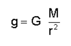
where (using metric):

g = acceleration due to gravity on the surface of the body (m/sec2)

G = universal gravitational constant = 6.672 x 10⁻¹¹ m3/kg/sec2

M = mass of the body (kg)

r = radius of the body (which is assumed to be spherical) (m)

You can determine the escape velocity from a body using the following equation:

Equation - Escape velocity

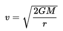
Applying these equations to the Earth and several smaller bodies in in the Solar System yields the following results:

g and escape velocity table

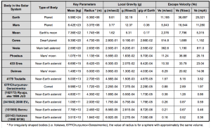
Note how weak the gravity is on the small bodies in this table. These are very different conditions than on the surface of the Moon or Mars where the low gravity still allows relatively conventional locomotion.

As noted in my 31 December 2015 post, the “U.S. Commercial Space Launch Competitiveness Act,” which was signed into law on 25 November 2015, opens the way for U.S. commercial exploitation of space, including commercial missions to asteroids and comets.  Let’s take a look at missions to these microgravity worlds and some of the unique issues associated with visiting a microgravity world.

2.  Recent and Current Missions to Asteroids and Comets

There have been several spacecraft that have made a successful rendezvous with one or more small bodies in the Solar System. Several have been fly-by missions. Four spacecraft have flown in close formation with or entered orbit around low-gravity bodies. Three of these missions included landing on (or at least touching) the body, and one returned very small samples to Earth. These missions are:

  • National Aeronautics and Space Administration’s (NASA) NEAR-Shoemaker
  • Japan Aerospace Exploration Agency’s (JAXA) Hayabusa
  • European Space Agency’s (ESA) Rosetta
  • NASA’s Dawn

In addition, China’s Chang’e 2 mission demonstrated its ability to navigate to an asteroid intercept after completing its primary mission in lunar orbit. JAXA’s Hayabusa 2 mission currently is enroute to asteroid rendezvous.

Following is a short synopsis of each of these missions.

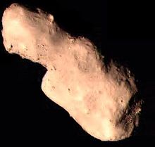
NASA’s NEAR-Shoemaker Mission (1996 – 2001): This mission was launched 17 February 1996 and on 27 June 1997 flew by the asteroid 253 Mathilde at a distance of about 1,200 km (746 miles).   On 14 February 2000, the spacecraft reached its destination and entered a near-circular orbit around the asteroid 433 Eros, which is about the size of Manhattan. After completing its survey of Eros, the NEAR spacecraft was maneuvered close to the surface and it touched down on 12 February 2001, after a four-hour descent, during which it transmitted 69 close-up images of the surface. Transmissions continued for a short time after landing. NEAR-Shoemaker was the first man-made object to soft-land on an asteroid.

Asteroid Eros                
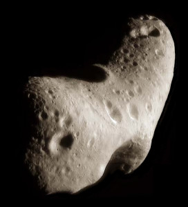
Asteroid EROS. Source: NASA/JPL/JHUAPL

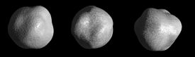
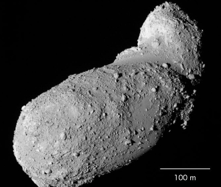
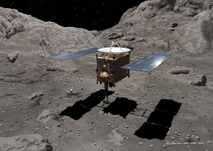
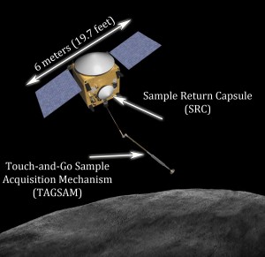
JAXA’s Hayabusa Mission (2003 – 2010): The Hayabusa spacecraft was launched in May 2003. This solar-powered, ion-driven spacecraft rendezvoused with near-Earth asteroid 25143 Itokawa in mid-September 2005.

Asteroid Itokawa           
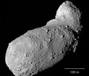
Asteroid Itokawa. Source: JAXA

Hayabusa carried the solar-powered MINERVA (Micro/Nano Experimental Robot Vehicle for Asteroid) mini-lander, which was designed to be released close to the asteroid, land softly, and move across the surface using an internal flywheel and braking system to generate the momentum needed to hop in microgravity. However, MINERVA was not captured by the asteroid’s gravity after being released and was lost in deep space.

In November 2005, Hayabusa moved in from its station-keeping position and briefly touched the asteroid to collect surface samples in the form of tiny grains of asteroid material.

Hayabusa taking a sampleHayabusa in position to obtain samples. Source: JAXA

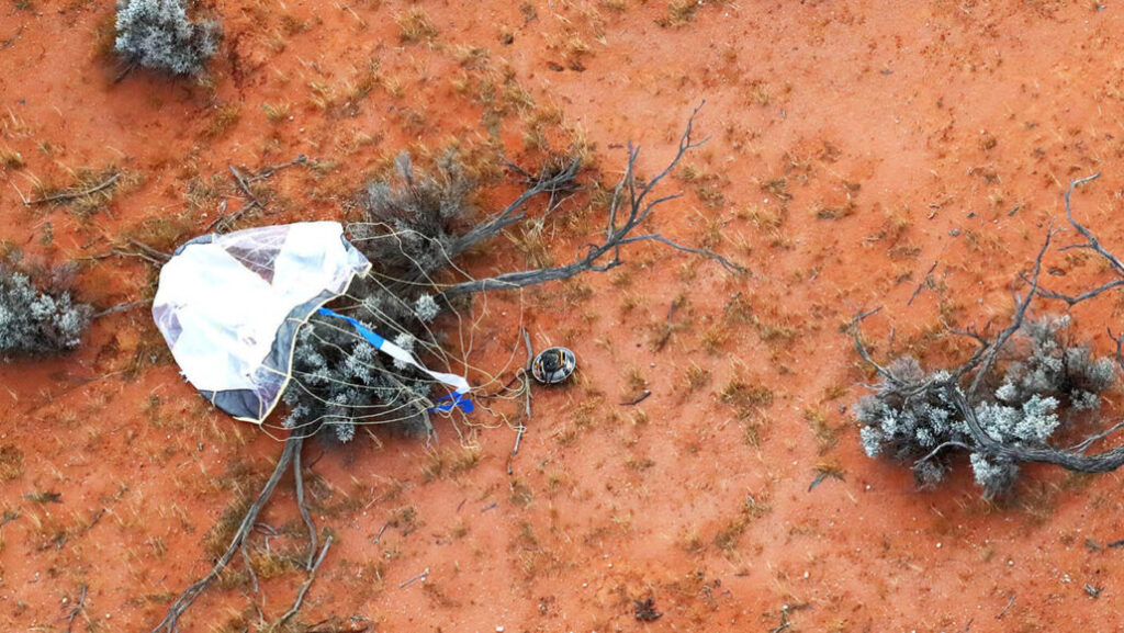
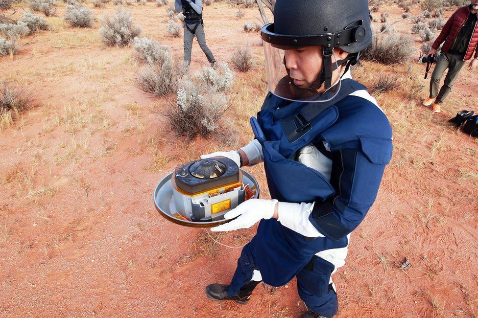
The spacecraft then backed off and navigated back to Earth using its failing ion thrusters. Hayabusa returned to Earth on 13 June 2010 and the sample-return capsule, with about 1,500 grains of asteroid material, was recovered after landing in the Woomera Test Range in the western Australian desert.

You’ll find a JAXA mission summary briefing at the following link:

https://www.nasa.gov/pdf/474206main_Kuninaka_HayabusaStatus_ExploreNOW.pdf

ESA’s Rosetta Mission (2004 – present): The Rosetta spacecraft was launched in March 2004 and in August 2014 rendezvoused with and achieved orbit around irregularly shaped comet 67P/Churyumov-Gerasimenko. This comet orbits the Sun outside of Earth’s orbit, between 1.24 and 5.68 AU (astronomical units; 1 AU = average distance from Earth’s orbit to the Sun). The size of 67P/Churyumov-Gerasimenko is compared to downtown Los Angeles in the following figure.
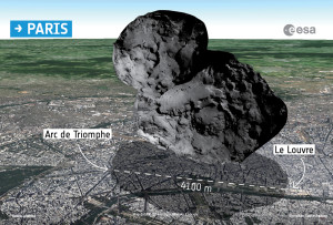
ESA Attempts To Land Probe On CometSource: ESA

Currently, Rosetta remains in orbit around this comet. The lander, Philae, is on the surface after a dramatic rebounding landing on 12 November 2014. Anchoring devices failed to secure Philae after its initial touchdown. The lander bounced twice and finally came to rest in an unfavorable position after contacting the surface a third time, about two hours after the initial touchdown. Philae was the first vehicle to land on a comet and it briefly transmitted data back from the surface of the comet in November 2014 and again in June – July 2015.

NASA’s Dawn Mission (2007 – present): Dawn was launched on 27 September 2007 and used its ion engine to fly a complex flight path to a 2009 gravitational assist flyby of Mars and then a rendezvous with the large asteroid Vesta (2011 – 2012) in the main asteroid belt.

NASA_Dawn_spacecraft_near_Ceres   
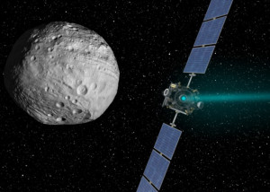
Dawn approaches Vesta. Source: NASA / JPL Caltech

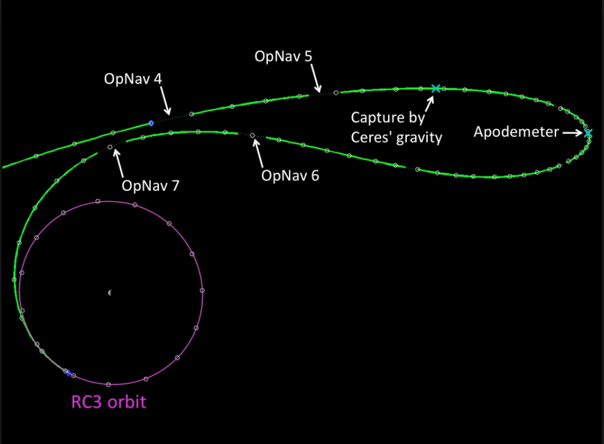
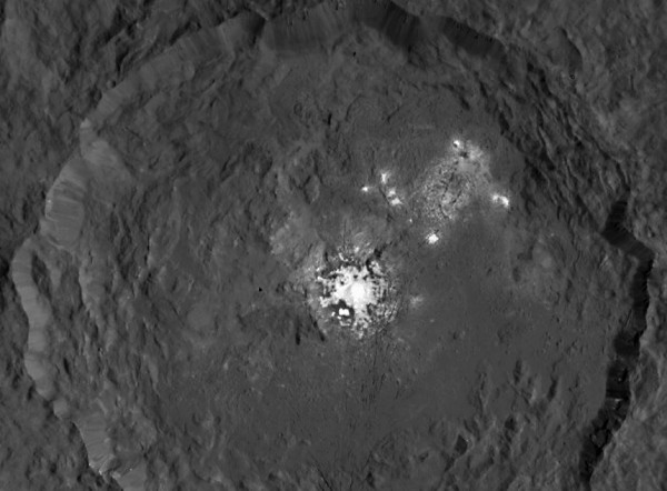
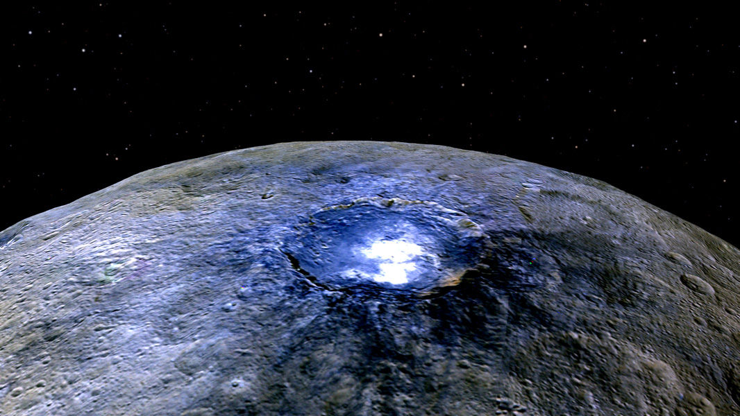
Dawn spent 14 months in orbit surveying Vesta before departing to its next destination, the dwarf planet Ceres, which also is in the main asteroid belt. On 6 March 2015 Dawn was captured by Ceres’ gravity and entered its initial orbit following the complex trajectory shown in the following diagram.

Dawn navigation to Ceres orbit   Dawn captured by Ceres gravity. Source: NASA / JPL Caltech

Dawn is continuing its mapping mission in a circular orbit at an altitude of 385 km (240 miles), circling Ceres every 5.4 hours at an orbital velocity of about 983 kph (611 mph). The Dawn mission does not include a lander.

See my 20 March 2015 and 13 Sep 2015 posts for more information on the Dawn mission.

CNSA’s Chang’e 2 extended mission (2010 – present): The China National Space Agency’s (CNSA) Chang’e 2 spacecraft was launched in October 2010 and placed into a 100 km lunar orbit with the primary objective of mapping the lunar surface. After completing this objective in 2011, Chang’e 2 navigated to the Earth-Sun L2 Lagrange point, which is a million miles from Earth in the opposite direction of the Sun. In April 2012, Chang’e 2 departed L2 for an extended mission to asteroid 4179 Toutatis, which it flew by in December 2012.

Toutatis_from_Chang'e_2
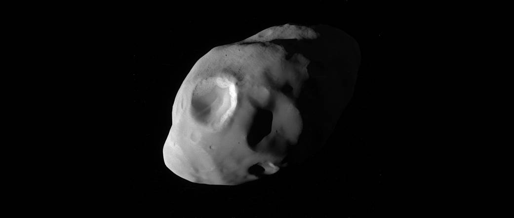
Asteroid Toutatis. Source: CHSA

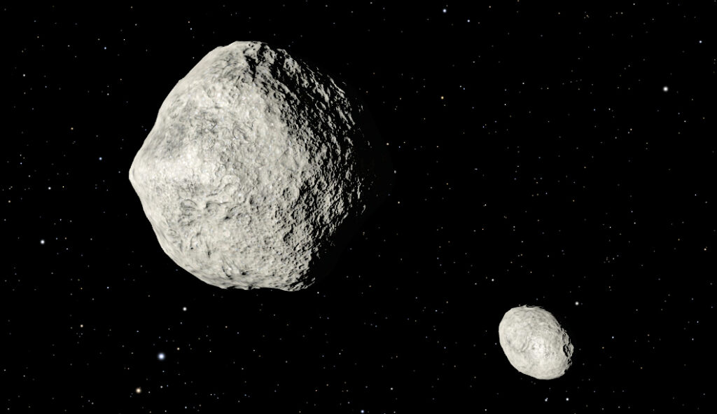
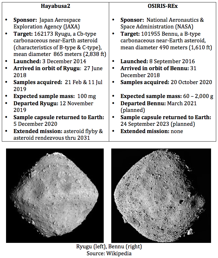
JAXA’s Hayabusa 2 Mission (2014 – 2020): The JAXA Hayabusa 2 spacecraft was launched on 3 December 2014. This ion-propelled spacecraft is very similar to the first Hayabusa spacecraft. Its planned arrival date at the target asteroid, 1999 JU3 (Ryugu), is in mid-2018.   As you can see in the following diagram, 1999 JU3 is a substantially larger asteroid than Itokawa.
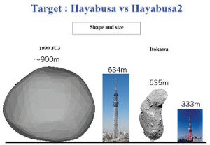
Hayabusa 1-2 target comparisonSource: JAXA

The spacecraft will spend about a year mapping the asteroid using Near Infrared Spectrometer (NIRS3) and Thermal Infrared Imager (TIR) instruments.

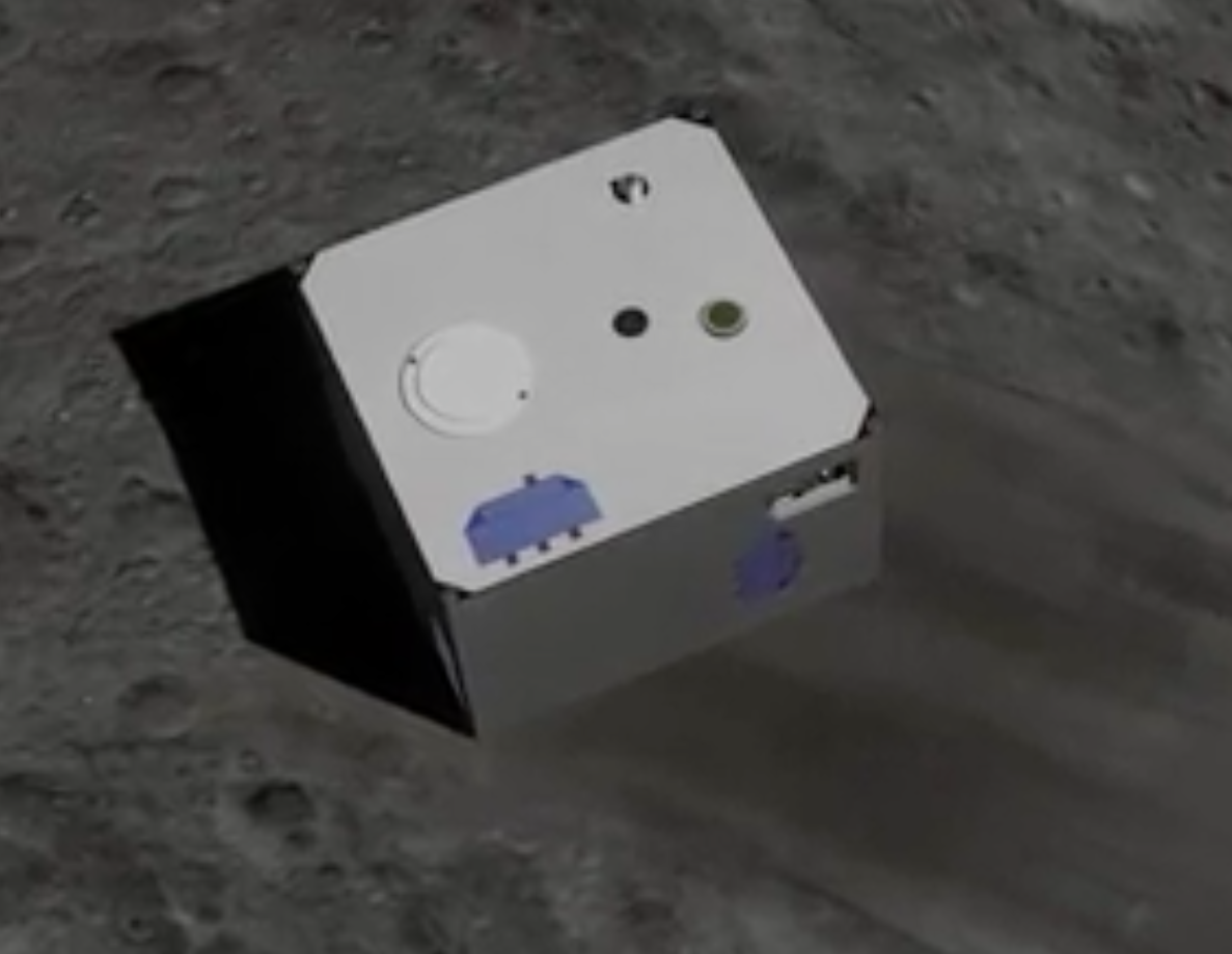
Hayabusa 2 includes three solar-powered MINERVA-II mini-landers and one battery-powered MASCOT (Mobile Asteroid Surface Scout) small lander. All landers will be deployed to the asteroid surface from an altitude of about 100 meters (328 feet) so they can be captured by the asteroid’s very weak gravity. The 1.6 – 2.5 kg (3.5 – 5.5 pounds) MINERVA-II landers will deliver imagery and temperature measurements. The 10 kg (22 pound) MASCOT will make measurements of surface composition and properties using a camera, magnetometer, radiometer, and infrared microscope. All landers are expected to make several hops to take measurements at different locations on the asteroid’s surface.

Three MINERVA landers

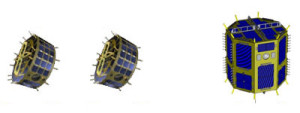
Three MINERVA mini-landers. Source: JAXA

MASCOT lander         
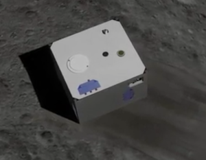
MASCOT small lander. Source: JAXA

For sample collection, Hayabusa 2 will descend to the surface to capture samples of the surface material. A device called a Small Carry-on Impactor (SCI) will be deployed and should impact the surface at about 2 km/sec, creating a small crater to expose material beneath the asteroid’s surface. Hayabusa 2 will attempt to gather a sample of the exposed material. More information about SCI is available at the following link:

http://www.lpi.usra.edu/meetings/lpsc2013/pdf/1904.pdf

At the end of 2019, Hayabusa 2 is scheduled to depart asteroid 1999 JU3 (Ryugu) and return to Earth in 2020 with the collected samples. You will find more information on the Hayabusa 2 mission at the JAXA website at the following links:

http://global.jaxa.jp/projects/sat/hayabusa2/

and,

http://www.lpi.usra.edu/sbag/meetings/jan2013/presentations/sbag8_presentations/TUES_0900_Hayabusa-2.pdf

3.  Future Missions:

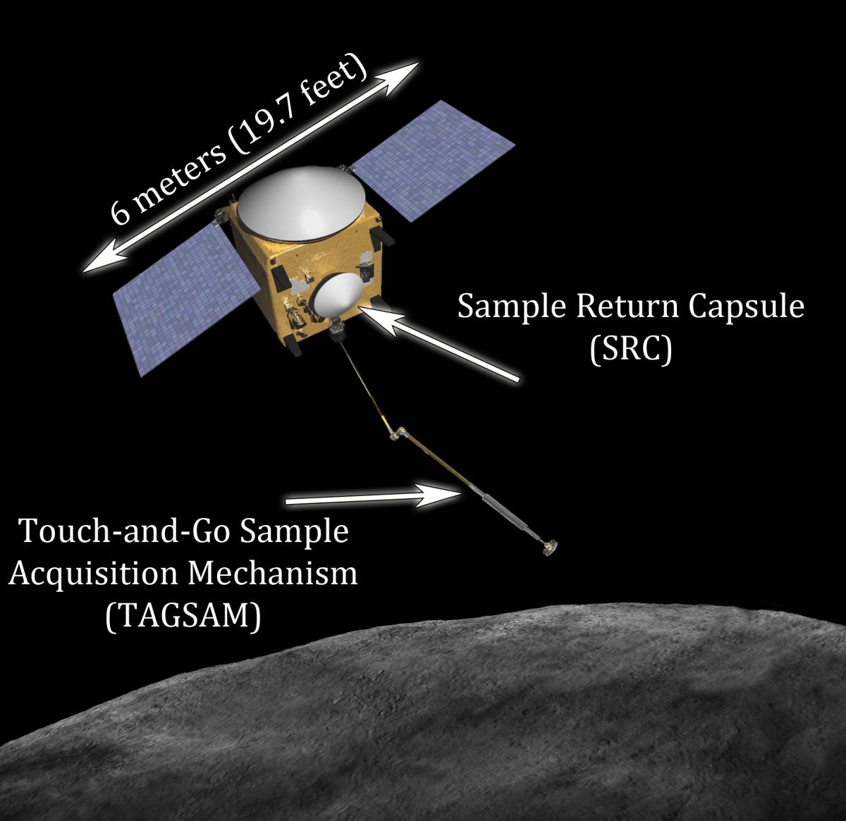
NASA OSIRIS-REx: This NASA’s mission is expected to launch in September 2016, travel to the near-Earth asteroid 101955 Bennu, map the surface, harvest a sample of surface material, and return the samples to Earth for study. After arriving at Bennu in 2018, the solar-powered OSIRIS-Rex spacecraft will map the asteroid surface from a station-keeping distance of about 5 km (3.1 miles) using two primary mapping instruments: the OVIRS Visible and Infrared Spectrometer and the OTRS Thermal Emission Spectrometer. Together, these instruments are expected to develop a comprehensive map of Bennu’s mineralogical and molecular components and enable mission planners to target the specific site(s) to be sampled. In 2019, a robotic arm on OSIRIS-REx will collect surface samples during one or more very close approaches, without landing. These samples (60 grams minimum) will be loaded into a small capsule that is scheduled to return to Earth in 2023.

OSIRIS-REx SpacecraftOSIRIS-REx spacecraft. Source: NASA / ASU

For more information on OSIRIS-REx, visit the NASA website at the following link:

http://sservi.nasa.gov/articles/nasas-asteroid-sample-return-mission-moves-into-development/

and the ASU website at the following link:

http://www.asteroidmission.org/objectives/

NASA Asteroid Redirect Mission (ARM): This mission will involve rendezvousing with a near-Earth asteroid, mapping the surface for about a year, and locating a suitable bolder to be captured [maximum diameter about 4 meters (13.1 feet)]. The ARM spacecraft will land and capture the intended bolder, lift off and deliver the bolder into a stable lunar orbit during the first half of the next decade. The current reference target is known as asteroid 2008 EV5.

ARM asteroid-capture      
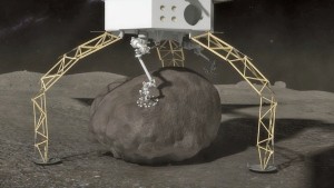
ARM lander gripping a bolder on an asteroid. Source: NASA

You can find more information on the NASA Asteroid Redirect Mission at the following links:

https://www.nasa.gov/content/what-is-nasa-s-asteroid-redirect-mission

and

https://www.nasa.gov/pdf/756122main_Asteroid%20Redirect%20Mission%20Reference%20Concept%20Description.pdf

4. Locomotion in Microgravity

OK, you’ve landed on a small asteroid, your spacecraft has anchored itself to the surface and now you want to go out and explore the surface. If this is asteroid 2008 EV5, the local gravity is about 1.79 E-05 that of Earth (less than 2/100,000 the gravity of Earth) and the escape velocity is about 0.6 mph (1 kph). Just how are you going to move about on the surface and not launch yourself on an escape trajectory into deep space?

There is a good article on the problems of locomotion in microgravity in a 7 March 2015 article entitled, “A Lightness of Being,” in the Economist magazine. You can find this article on the Economist website at the following link:

http://www.economist.com/news/technology-quarterly/21645508-space-vehicles-can-operate-ultra-low-gravity-asteroids-and-comets-are

In this article, it is noted that:

“Wheeled and tracked rovers could probably be made to work in gravity as low as a hundredth of that on Earth……But in the far weaker microgravity of small bodies like asteroids and comets, they would fail to get a grip in fine regolith. Wheels also might hover above the ground, spinning hopelessly and using up power. So an entirely different system of locomotion is needed for rovers operating in a microgravity.”

Novel concepts for locomotion in microgravity include:

  • Hoppers / tumblers
  • Structurally compliant rollers
  • Grippers

Hoppers / tumblers: Hoppers are designed to move across a surface using a moving internal mass that can be controlled to transfer momentum to the body of the rover to cause it to tumble or to generate a more dramatic hop, which is a short ballistic trajectory in microgravity. The magnitude of the hop must be controlled so the lander does not exceed escape velocity during a hop. JAXA’s MINERVA-II and MASCOT asteroid landers both are hoppers.

JAXA described the MINERVA-II hopping mechanism as follows:

“MINERVA can hop from one location to another using two DC motors – the first serving as a torquer, rotating an internal mass that leads to a resulting force, sufficient to make the rover hop for several meters. The second motor rotates the table on which the torquer is placed in order to control the direction of the hop. The rover reaches a top speed of 9 centimeters per second, allowing it to hop a considerable distance.”

JAXA MINERVA hopper
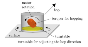
MINERVA torque & turntable. Source: JAXA

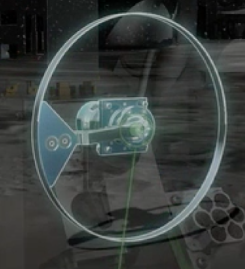
The MASCOT hopper operates on a different principle:

“With a mass of not even half a gram in the gravitational field of the asteroid, the (MASCOT) lander can easily withstand its initial contact with the surface and several bounces that are expected upon landing. It also means that only small forces are needed to move the lander from point to point. MASCOT’s Mobility System essentially consists of an off-centered mass installed on an eccentric arm that moves that mass to generate momentum that is sufficient to either rotate the lander to face the surface with its instruments or initiate a hop of up to 70 meters to get to the next sampling site.”

MASCOT Mobility SystemMASCOT mobility mechanism. Source: JAXA

You will find a good animation of MASCOT and its Mobility System at the following link:

http://www.dlr.de/dlr/en/desktopdefault.aspx/tabid-10081/151_read-18664/#/gallery/23722

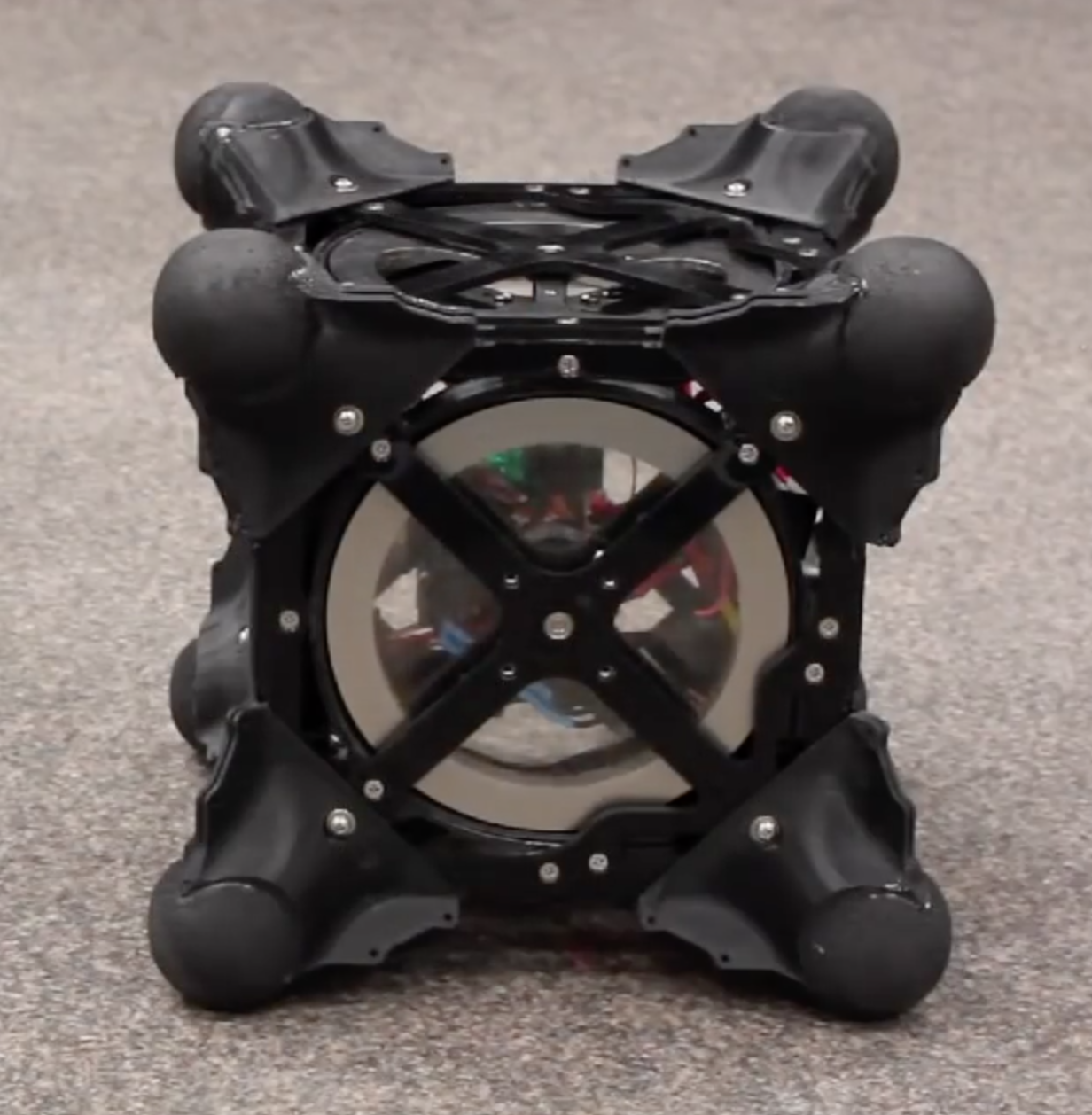
NASA is examining a class of microgravity rovers called “hedgehogs” that are designed to hop and tumble on microgravity surfaces by spinning and braking a set of three internal flywheels. Cushions or spikes at the corners of the cubic body of a hedgehog protect the body from the terrain and act as feet while hopping and tumbling.

NASA Hedgehog                               
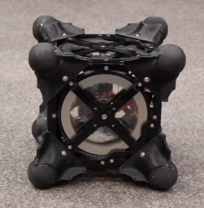
NASA Hedgehog prototype. Source: NASA

Read more on the NASA hedgehog rovers at the following link:

http://www.jpl.nasa.gov/news/news.php?feature=4712

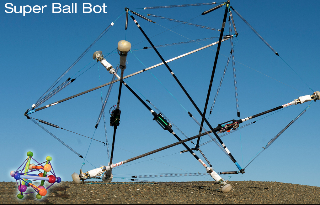
Structurally compliant rollers: One means of “rolling” across a microgravity surface is with a deformable structure that allows the location of the center of mass to be controlled in a way that causes the rover to tip over in the desired direction of motion. NASA is exploring the use of a class of rolling rovers called Super Ball Bots, which are terrestrial rovers based on a R. Buckminster Fuller’s tensegrity toy. NASA explains:

“The Super Ball Bot has a sphere-like matrix of cables and joints that could withstand being dropped from a spacecraft high above a planetary surface and hit the ground with a bounce. Once on the planet, the joints could adjust to roll the bot in any direction while housing a data collecting device within its core.”

NASA Super Ball Bot                    Source: http://www.nasa.gov/content/super-ball-bot

You’ll find a detailed description of the principles behind tensegrity (tensional integrity) in a 1961 R. Buckminster Fuller paper at the following link:

http://www.rwgrayprojects.com/rbfnotes/fpapers/tensegrity/tenseg01.html

Grippers: Without having a grip on a microgravity body, a rover cannot use sampling tools that generate a reaction force on the rover (i.e., drills, grinders, chippers). For such operations to be successful a rover needs an anchoring system to secure the rover and transfer the reaction loads into the microgravity body.

An approach being developed by Jet Propulsion Laboratory (JPL) involves articulated feet with microspine grippers that have a large number of small claws that can grip irregular rocky surfaces.

JPL microspine gripper           
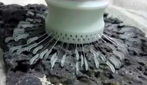
Microspine gripper. Source: NASA / JPL

Such a gripper could be used to hold a rover in place during mechanical sampling activities or to allow a rover to climb across an irregular surface like a spider.  See more about the operation of the NASA / JPL microspine gripper at the following link:

https://www-robotics.jpl.nasa.gov/tasks/taskVideo.cfm?TaskID=206&tdaID=700015&Video=147

5. Conclusions

Missions to small bodies in our Solar System are very complex undertakings that require very advanced technologies in many areas, including: propulsion, navigation, autonomous controls, remote sensing, and locomotion in microgravity. The ambitious current and planned future missions will greatly expand our knowledge of these small bodies and the engineering required to operate spacecraft in their vicinity and on their surface.

While commercial exploitation of dwarf planets, asteroids and comets still may sound like science fiction, the technical foundation for such activities is being developed now. It’s hard to guess how much progress will be made in the next decades. However, I’m convinced that the “U.S. Commercial Space Launch Competitiveness Act,” will encourage commercial investments in space exploration and exploitation and lead to much greater progress than if we depended on NASA alone.

The technologies being developed also may lead, in the long term, to effective techniques for redirecting an asteroid or comet that poses a threat to Earth. Such a development would give our Planetary Defense Officer (see my 21 January 2016 post) an actual tool for defending the planet.

The Bright Spots on Ceres Come into Focus

Peter Lobner

In my 20 March 2015 post, I discussed the Dawn spacecraft mission to the large asteroid Vesta and the dwarf planet Ceres, both of which are in the main asteroid belt between Mars and Jupiter. Dawn arrived in orbit around Ceres on 6 March 2015, at an initial altitude of 8,400 miles (13,518 kilometers). On approach and from this high altitude orbit, Dawn photographed two very bright spots on the surface of Ceres.

Ceres seen from Dawn  Source: NASA

After spending six months mapping the surface of Ceres and gradually descending to lower altitude orbits, Dawn currently is in a much lower “high-altitude mapping orbit” (HAMO) at 915 miles (1,470 kilometers) above the surface. Ceres’ diameter is about 587 miles (946 kilometers). Due to the low mass of this dwarf planet, Dawn’s orbital speed in the HAMO is only 400 mph (645 kph). The spacecraft completes one orbit in about 19 hours.

From its current vantage point in HAMO, Dawn has provided a much better view of the bright spots on Ceres. The following composite photo shows the bright spots at a resolution of 450 feet (140 meters) per pixel.

ceres-bright-spots-Sep2015,jpg  Source: NASA

The source of the bright spots has not yet been determined. We’ll get a more detailed view later in 2015, when the spacecraft descends to the “low altitude mapping orbit” (LAMO) at an altitude of 230 miles (370 kilometers).

You can keep up with the work of the Dawn project team at the following NASA / Jet Propulsion Lab website:

http://dawnblog.jpl.nasa.gov

 9 December 2015 Update:

NASA’s Jet Propulsion Laboratory (JPL) released closeup photos of the bright spots, which appear to be globally distributed on Ceres. JPL scientists reported that Ceres has more than 130 bright areas, and most of them appear to be associated with impact craters.   There is evidence that the bright spots may be salt deposits left behind after a subterranean briny water-ice deposit was exposed by an impact and the  ice-water sublimated into space.  Here is a closeup, false-color photo of the Occator Crater, emphasizing the deposits of bright material on the crater floor.

Occator Crater - Ceres_JPL

You can read more on this subject on the JPL website at the following link:

http://www.jpl.nasa.gov/news/news.php?feature=4785

1 November 2018 Update:

On 1 November 2018, NASA reported the end of the Dawn mission:

“Dawn missed scheduled communications sessions with NASA’s Deep Space Network on Wednesday, Oct. 31, and Thursday, Nov. 1. After the flight team eliminated other possible causes for the missed communications, mission managers concluded that the spacecraft finally ran out of hydrazine, the fuel that enables the spacecraft to control its pointing. Dawn can no longer keep its antennae trained on Earth to communicate with mission control or turn its solar panels to the Sun to recharge.”

You’ll find more information about the Dawn mission and its many accomplishments on the NASA / JPL website at the following link:

https://dawn.jpl.nasa.gov/news/news-detail.html?id=7275

New Horizons Spacecraft Rapidly Approaching Encounter with Pluto

Peter Lobner

New Horizons is rapidly approaching Pluto for a fast fly-by encounter with closest approach at 7:49 am on Tuesday, 14 July 2015. You’ll find basic information about the New Horizons mission in my 14 March 2015 post on this subject. Detailed information is available at the NASA New Horizons mission website at the following link:

https://www.nasa.gov/mission_pages/newhorizons/main/index.html

The spacecraft will fly past Pluto at 30,800 mph (49,600 kph), and is expected to fly within 7,750 miles (11,265 km) of Pluto’s surface. The close-encounter segment of the flyby is quite brief, as shown in the following diagram of New Horizon’s trajectory through the Pluto system.

New Horizons trajectorySource: NASA/Applied Physics Laboratory/Southwest Research Institute

On 9 July, New Horizon’s Long Range Reconnaissance Imager (Lorri) took the following photo from a range of 3.3 million miles. Some basic surface features have been noted by the NASA project team, along with a diagram indicating Pluto’s north pole, equator, and central meridian.

Pluto pic 1

Source: NASA/Applied Physics Laboratory/Southwest Research Institute

On 11 July, the project team released the following slightly more detailed photo that reveals linear features that may be cliffs, as well as a circular feature that could be an impact crater.

Pluto pic 2

Source: NASA/Applied Physics Laboratory/Southwest Research Institute

Below is a photo released on 9 July showing both Pluto and it’s largest moon, Charon, which orbit each other around their common center of gravity. You’ll find more information on the unusual orbital interactions among Pluto and it’s five known moons in my 6 June 2015 post on that subject.

Pluto pic 3

Source: NASA/Applied Physics Laboratory/Southwest Research Institute

Messenger Spacecraft Mission at Mercury About to End

Peter Lobner

Updated 12 January 2016

The 1,069 pound Messenger (MErcury Surface, Space ENvironment, GEochemistry, and Ranging) spacecraft is only the second spacecraft sent to Mercury. Mariner 10 flew past Mercury three times in 1974 and 1975. Messenger was launched on 3 August 2004 and flew for 6-1/2 years on a circuitous trajectory that included 15 orbits of the sun, one flyby of Earth, two flybys of Venus, and three flybys of Mercury before entering orbit around Mercury in 18 March 2011. The series of planetary flybys allowed Messenger to decelerate relative to Mercury and achieve orbit with minimal use of fuel.

The NASA Messenger mission website is at the following link:

http://www.nasa.gov/mission_pages/messenger/main/index.html

Messenger is solar-powered, with its science payload and propulsion system located behind a sunshade to protect against the intense solar radiation encountered at Mercury’s close orbit of the Sun.

image  Source: Johns Hopkins University/APL

Messenger has instrumentation for mapping and characterizing Mercury using imaging cameras, laser altimeter, various spectrometers, magnetometer, and a radio science package to measure slight velocity changes in orbit. You can read details on the spacecraft instrumentation systems at the following link:

http://messenger.jhuapl.edu/the_mission/spacecraft_design.html

After four years in orbit, fuel needed to maintain orbit is expected to be depleted in April. Messenger’s orbit will decay and the spacecraft eventually will crash at perigee into Mercury’s surface at its orbital speed of 8,750 mph.

12 January 2016 update:

On 30 April 2015, Messenger crashed into the surface of Mercury on the side facing away from Earth.  Before crashing, Messenger orbited Mercury 4,105 times and collected more than 277,000 images.  A composite photograph of Mercury created from thousands of Messenger images is shown below:

Mercury composite imaages from MessengerSource: NASA /  Johns Hopkins University/APL