All posts by Drummer

Energy Literacy

January 27, 2017All Posts, Energy, Power Generating Technology - Alternate, Power Generating Technology - Fossil, Power Generating Technology - Nuclear, STEM Education, Transportationenergy efficiency, energy literacy, energy sources, energy utilizationDrummer

Peter Lobner

I was impressed in 2007 by the following chart in Scientific American, which shows where our energy in the U.S. comes from and how the energy is used in electricity generation and in four consumer sectors. One conclusion is that more than half of our energy is wasted, which is clearly shown in the bottom right corner of the chart. However, this result shouldn’t be surprising.

Source: Scientific American / Jen Christiansen, using LLNL & DOE 2007 data

The waste energy primarily arises from the efficiencies of the various energy conversion cycles being used. For example, the following 2003 chart shows the relative generating efficiencies of a wide range of electric power sources. You can see in the chart that there is a big plateau at 40% efficiency for many types of thermal cycle power plants. That means that 60% of the energy they used is lost as waste heat. The latest combined cycle plants have demonstrated net efficiencies as high as 62.22% (Bouchain, France, 2016, see details in my updated 17 March 2015 post, “Efficiency in Electricity Generation”).

Source: Eurelectric and VGB PowerTech, July 2003

Another source of waste is line loss in electricity transmission and distribution from generators to the end-users. The U.S. Energy Information Administration (EIA) estimates that electricity transmission and distribution losses average about 6% of the electricity that is transmitted and distributed.

There is an expanded, interactive, zoomable map of U.S. energy data that goes far beyond the 2007 Scientific American chart shown above. You can access this interactive map at the following link:

http://energyliteracy.com

The interactivity in the map is impressive, and the way it’s implemented encourages exploration of the data in the map. You can drill down on individual features and you can explore particular paths in much greater detail than you could in a physical chart containing the same information. Below are two example screenshots. The first screenshot is a top-level view. As in the Scientific American chart, energy sources are on the left and final disposition as energy services or waste energy is on the right. Note that waste energy is on the top right of the interactive map.

The second screenshot is a more detailed view of natural gas production and utilization.

As reported by Lulu Chang on the digitaltrends.com website, this interactive map was created by Saul Griffith at the firm Otherlab (https://otherlab.com). You can read her post at the following link:

http://www.digitaltrends.com/home/otherlab-energy-chart/

I hope you enjoy exploring the interactive energy literacy map.

Protocol for Reporting UFO Sightings

January 26, 2017Aeronautical, All Posts, National SecurityAir Force Letter AFL 200-5, Air Force Regulation AFR 200-2, Air Force Regulation AFR 80-17, FLYOBRPTS, Project Blue Book, Project Grudge, Project Sign, UFO, unidentified flying object, USAF letter AFOIN-C/CC-2Drummer

Peter Lobner

The United States Air Force began investigating unidentified flying objects (UFOs) in the fall of 1947 under a program called Project Sign, which later became Project Grudge, and in January 1952 became Project Blue Book. As you might expect, the USAF developed a reporting protocol for these projects.

Starting in 1951, the succession of Air Force documents that provided UFO reporting guidance is summarized below:

Headquarters USAF Letter AFOIN-C/CC-2

This letter, entitled, “Reporting of Information on Unidentified Flying Objects,” dated 19 December 1951, may be the original guidance document for UFO reporting. So far, I have been unable to find a copy of this document. The Project Blue Book archives contain examples of UFO reports from 1952 citing AFOIN-C/CC-2.

Air Force Letter AFL 200-5

The first reporting protocol I could find was Air Force Letter AFL 200-5, “Unidentified Flying Objects Reporting,” dated 29 April 1952, which was issued on behalf of the Secretary of the USAF by Hoyt S. Vandenberg, Chief of Staff of the USAF.

Defines UFOs as, “any airborne object which by performance, aerodynamic characteristics, or unusual features, does not conform to any presently known aircraft or missile type.”
UFO reporting is treated as an Intelligence activity (denoted by the 200-series document number)
Provides brief guidance on report content, which was to be submitted on AF Form 112, “Air Intelligence Information Report,” and not classified higher than RESTRICTED.
The local Commanding Officer is responsible for forwarding FLYOBRPTS to the appropriate agencies. FLYOBRPT is an acronym for FLYing OBject RePorT.
Responsibility for investigating UFOs was assigned to the Air Technical Intelligence Center (ATIC) at Wright Patterson Air Force Base, Ohio. ATIC was a field activity of the Directorate of Intelligence in USAF Headquarters.
AFL 200-5 does not indicate that it superseded any prior USAF UFO reporting guidance document, but it is likely that it replaced USAF letter AFOIN-C/CC-2, dated 19 December 1951.

Download AFL 200-5 at the following link:

http://www.cufon.org/cufon/AFL_200-5.pdf

How to Make FLYOBRPTs

In 1953, the AITC issued “How to Make FLYOBRPTs,” dated 25 July 1953, to help improve reporting required by AFL 200-5.

Source: USAF

This guidance document provides an interesting narrative about UFOs through 1953, explains how to collect information on a UFO sighting, including interacting with the public during the investigation, and how to complete a FLYOBRPT using four detailed data collection forms.

Ground Observer’s Information Sheet (9 pages)
Electronics Data Sheet (radar) (5 pages)
Airborne Observer’s Data Sheet (9 pages) and,
Supporting Data form (8 pages)

This report showed that the USAF had a sense of humor about UFO reporting.

Source: USAF

Download “How to Make FLYOBRPTs” at the following link:

http://www.cufon.org/cufon/FLYOBRPT.pdf

Air Force Regulation AFR 200-2

In 1953, the Secretary of the Air Force, Harold E. Talbott, issued the original Air Force Regulation AFR 200-2, “Unidentified Flying Objects Reporting”, dated 26 August 1953.

Superseded AFL 200-5, dated 29 April 1952
Defines procedures for reporting UFOs and restrictions on public discussion by Air Force personnel
Change 200-2A was issued on 2 November 1953
Between 1954 and 1962, the USAF issued several subsequent versions of AFR 200-2, as listed below.

AFR 200-2, “Unidentified Flying Objects Reporting (Short Title: FLYOBRPT)”, dated 12 August 1954.

Superseded AFR 200-2 dated 26 August 1953 and Change 200-2A
Identifies the USAF interest in UFOs as follows: “Air Force interest in unidentified flying objects is twofold: First as a possible threat to the security of the United States and its forces, and secondly, to determine technical aspects involved.”
Defines an expected report format that is less comprehensive than the guidance in “How to Make FLYOBRPTs.”
Clarifies that Headquarters USAF will release summaries of evaluated data to the public. Also notes that it is permissible to respond to local inquiries when the object is positively identified as a “familiar object” (not a UFO). In other cases, the only response is that ATIC will analyze the data.
Download this version of AFR 200-2 at the following link:

http://www.cufon.org/cufon/afr200-2.htm

AFR 200-2, “Unidentified Flying Objects (UFO),” dated 5 February 1958

Supersedes the version dated 12 August 1954
Broadens the USAF interest in UFOs: “First as a possible threat to the security of the United States and its forces; second, to determine the technical or scientific characteristics of any such UFOs; third, to explain or identify all UFO sightings…”
Updates report formats and provides additional guidance on reporting
Download this version from the CIA website at the following link:

https://www.cia.gov/library/readingroom/docs/CIA-RDP81R00560R000100040072-9.pdf

AFR 200-2, “Unidentified Flying Objects (UFO),” dated 14 September 1959

Supersedes the version dated 5 February 1958

AFR 200-2, “Unidentified Flying Objects (UFO),” dated 20 July 1962

Supersedes the version dated 14 September 1959
Superseded by AFR 80-17

Air Force Regulation AFR 80-17

In 1966, the USAF issued AFR 80-17, “Unidentified Flying Objects (UFO),” dated 19 September 1966

Supersedes AFR 200-2 dated 20 July 1962.
Two changes were issued:
- AFR 80-17, Change 80-17A, dated 8 November 1966
- AFR 80-17, Change 1, dated 26 October 1968, superseded AFR 80-17A, 8 November 1966
No longer considers UFO reporting as an intelligence activity, as denoted by the 80-series number assigned to the AFR
Places UFO reporting under the Research and Development Command. This is consistent with recasting ATIC into the Foreign Technology Division (FTD) of the Air Force Systems Command at Wright-Patterson AFB.
Broadly redefines UFO as “any aerial phenomenon which is unknown or appears out of the ordinary to the observer.”
Orders all Air Force bases to provide an investigative capability
Change 80-17A assigned University of Colorado to conduct an independent scientific investigation of UFOs. Physicist Edward U. Condon would direct this work.

Download AFR 80-17, with change 80-17A and change 1 here:

http://www.cufon.org/cufon/afr80-17.htm

Project Blue Book’s final report

In late October 1968, the University of Colorado’s final report was completed and submitted for review by a panel of the National Academy of Sciences. The panel approved of the methodology and concurred with Edward Condon’s conclusion:

“That nothing has come from the study of UFOs in the past 21 years that has added to scientific knowledge. Careful consideration of the record as it is available to us leads us to conclude that further extensive study of UFOs probably cannot be justified in the expectation that science will be advanced thereby.”

In January 1969, a 965-page paperback version of the report was published under the title, “Scientific Study of Unidentified Flying Objects.”

On 17 December 1969, Air Force Secretary Robert C. Seamans, Jr., announced the termination of Project Blue Book.

Additional resources

You’ll find a good history by of the U.S. Air Force UFO programs written by Thomas Tulien at the following link:

http://sohp.us/history-of-the-usaf-ufo-programs/8-turning-point.php

Doomsday Clock Reset

January 26, 2017All Posts, Biotechnology, Cyber Security, Global Climate, National Security, Nuclear Arms & Arms ControlBulletin of the Atomic Scientists, Doomsday ClockDrummer

Peter Lobner

This year is the 70^th anniversary of the Doomsday Clock, which the Bulletin of the Atomic Scientists describes as follows:

“The Doomsday Clock is a design that warns the public about how close we are to destroying our world with dangerous technologies of our own making. It is a metaphor, a reminder of the perils we must address if we are to survive on the planet.”

You’ll find an overview on the Doomsday Clock here:

http://thebulletin.org/overview

The Clock was last changed in 2015 from five to three minutes to midnight. In January 2016, the Doomsday Clock’s minute hand did not change.

On 26 January 2017, the Bulletin of the Atomic Scientists Science and Security Board, in consultation with its Board of Sponsors, which includes 15 Nobel Laureates, decided to reset the Doomsday Clock to 2-1/2 minutes to midnight. This is the closest it has been to midnight in 64 years, since the early days of above ground nuclear device testing.

The Science and Security Board warned:

“In 2017, we find the danger to be even greater (than in 2015 and 2016), the need for action more urgent. It is two and a half minutes to midnight, the Clock is ticking, global danger looms. Wise public officials should act immediately, guiding humanity away from the brink. If they do not, wise citizens must step forward and lead the way.”

You can read the Science and Security Board’s complete statement at the following link:

http://thebulletin.org/sites/default/files/Final%202017%20Clock%20Statement.pdf

Their rationale for resetting the clock is not based on a single issue, but rather, the aggregate effects of the following issues, as described in their statement:

A dangerous nuclear situation on multiple fronts

Stockpile modernization by current nuclear powers, particularly the U.S. and Russia, has the potential to grow rather than reduce worldwide nuclear arsenals
Stagnation in nuclear arms control
Continuing tensions between nuclear-armed India and Pakistan
North Korea’s continuing nuclear development
The Iran nuclear deal has been successful in accomplishing its goals in its first year, but its future is in doubt under the new U.S. administration
Careless rhetoric about nuclear weapons is destabilizing; for example, the U.S. administration’s suggestion that South Korea and Japan acquire their own nuclear weapons to counter North Korea

The clear need for climate action

The Paris Agreement went into effect in 2016
Continued warming of the world was measured in 2016
S. administration needs to make a clear, unequivocal statement that it accepts climate change, caused by human activity, as a scientific reality

Nuclear power: An option worth careful consideration

Nuclear power a tempting part of the solution to the climate change problem
The scale of new nuclear power plant construction does not match the need for clean energy
In the short to medium term, governments should discourage the premature closure of existing reactors that are safe and economically viable
In the longer term, deploy new types of reactors that can be built quickly and are at least as safe as the commercial nuclear plants now operating
Deal responsibly with safety issues and with the commercial nuclear waste problem

Potential threats from emerging technologies

Technology continues to outpace humanity’s capacity to control it
Cyber attacks can undermining belief in representative government and thereby endangering humanity as a whole
Autonomous machine systems open up a new set of risks that require thoughtful management
Advances in synthetic biology, including the Crispr gene-editing tool, have great positive potential, but also can be misused to create bioweapons and other dangerous manipulations of genetic material
Potentially existential threats posed by a host of rapidly emerging technologies need to be monitored, and to the extent possible anticipated and managed.

Reducing risk: Expert advice

The Board is extremely concerned about the willingness of governments around the world— including the incoming U.S. administration—to ignore or discount sound science and considered expertise during their decision-making processes

Prior to the formal decision on the 2017 setting of the Doomsday Clock, the Bulletin took a poll to determine public sentiment on what the setting should be. Here are the results of this public pole.

How would you have voted?

Grand Finale of the Cassini Mission to Saturn

January 25, 2017All Posts, Planetary science, Spacecraft and MissionsCassini, ESA, European Space Agency, Huygens, NASA, National Aeronautics and Space AdministrationDrummer

Peter Lobner

The National Aeronautics and Space Administration’s (NASA’s) Cassini spacecraft was launched on 15 October 1997 and cruised through interplanetary space for seven years before arriving at Saturn on 30 June 2004. The Cassini spacecraft carried the European Space Agency’s (ESA’s) Huygens probe, which landed on Saturn’s largest moon, Titan, on 14 January 2005. Since then, Cassini has been performing a series of missions in orbit around Saturn, returning spectacular images and collecting scientific data on the ringed planet and its many moons.

In 2017, Cassini is performing its Grand Finale in a highly elliptical polar orbit around Saturn. The geometry for this orbital flight path is shown in the following diagram.

Source: NASA/JPL-Caltech

In the first phase of the Grand Finale (grey orbits in the above diagram), which is underway now, Cassini’s orbit crosses the plane of Saturn’s equatorial ring system just outside the F-ring (there are just two rings outside of the F-ring: G and E). Later in 2017, Cassini’s polar orbit will be adjusted to cross the plane of the ring system insider the innermost D-ring (blue orbits). From there the spacecraft will gradually descend toward Saturn in a region that has never before been explored. The mission will end when Cassini is destroyed somewhere in Saturn’s atmosphere (orange orbit). This is scheduled to occur on September 15, 2017 at 5:07 a.m. PDT.

NASA’s Cassini mission website is at the following link:

https://www.nasa.gov/mission_pages/cassini/main/index.html

You’ll find a NASA fact sheet on the Grand Finale here:

https://saturn.jpl.nasa.gov/legacy/files/Cassini_Grand_Finale_Fact_Sheet_508.pdf

You can follow the countdown to the final plunge into Saturn’s atmosphere and also review the entire mission timeline and other resources here:

https://saturn.jpl.nasa.gov/the-journey/timeline/#the-grand-finale

A few Grand Finale images taken during recent ring-grazing orbits past the F-ring are shown below. The source of these three images and captions are: NASA/JPL-Caltech/Space Science Institute

The above image, taken 16 January 2017, shows Saturn’s moon Daphnis (5 miles, 8 kilometers across), which orbits within the 26 mile (42 km) wide Keeler Gap (between the F and A rings). The gap appears foreshortened because of the viewing angle. The little moon’s gravity raises waves in the edges of the gap in both the horizontal and vertical directions.

Waves created by Daphnis are visible in this wider-angle view of the ring system. The F-ring is the bright, narrow ring crossing the center of the image. Since the moon moves in and out of the ring-plane, and closer to and farther from the rings’ edges as it orbits, the waves it makes change over time.

This image, taken on 18 December 2016, is one of the highest-resolution views ever taken of Saturn’s moon Pandora (52 miles, 84 kilometers across), which orbits just outside the F-ring.

13 April 2017 Update – Cassini’s close-up view of Saturn’s moon Pan

In early March, Cassini imaged Pan, which is one of Saturn’s innermost moons. As you can see in the following photos, this small moon (diameter of 221.7 miles, 35 km) has a most unusual shape. It isn’t known if the ridge circling the moon is solid, or a loose aggregation of particles with a very steep slope enabled by the moons weak gravity.

Source: NASA/JPL-Caltech/Space Science Institute

The NASA announcement and more photos of Pan are at the following link:

https://www.nasa.gov/image-feature/jpl/cassini-reveals-strange-shape-of-saturns-moon-pan

The Black Hole at our Galactic Center is Revealed Through Animations

January 24, 2017All Posts, Astronomy, Astrophysicsadaptive optics, European Extremely Large Telescope, European Southern Observatory, New Technology Telescope, Sagittarius A*, supermassive black hole, Thirty Meter Telescope, UCLA Galactic Center Group, Very Large Telescope, W.M. Keck ObservatoryDrummer

Peter Lobner

Evidence is mounting that a supermassive black hole named Sagittarius A* (Sagittarius A star) dominates the center of our Milky Way galaxy. Long-term observations of the galactic center by teams of astronomers are refining our understanding of how stars move in relation to this unseen black hole.

European Southern Observatory (ESO) observations of the galactic center

The ESO, which has many observatories located high in the mountains of northern Chile, has a team involved in observing our galactic center. Two of the ESO optical observatories used in this effort are:

New Technology Telescope (NTT), at the La Silla Observatory, has a 3.58 m (11.75 ft) main mirror. In 1989, NTT became the first astronomical observatory with adaptive optics to help correct for atmospheric distortion.
Very Large Telescope (VLT), which consists of four Unit Telescopes with 8.2 m (26.9 ft) diameter main mirrors and adaptive optics. The telescopes can work together, to form a giant ‘interferometer’, allowing astronomers to see details up to 25 times finer than with the individual Unit Telescopes.

On 10 December 2008, ESO issued a “science release” entitled, ”Unprecedented 16-Year Long Study Tracks Stars Orbiting Milky Way Black Hole,” which summarized the results of observations made at NTT and VLT from 1992 to 2008. This study mapped the orbits of 30 stars in the region around the galactic center (and did not use VLT’s interferometric capabilities).

Stars near our galactic center and the Sagittarius A* black hole. Source: eso0846 Science Release

The eso0846 science release is available at the following link:

http://www.eso.org/public/usa/news/eso0846/

In connection with this study, the ESO team also created a time-lapse video showing star motion around the Sagittarius A* black hole.

“Here, actual images, collected over the past 16 years, have been assembled into a time-lapse video. The real motion of the stars has been accelerated by a factor 32 million.”

This time-lapse video covers the central part of the above color image of the galactic center and shows stars moving around central point that is likely to be the black hole. You can see this animated sequence at the following link:

http://www.eso.org/public/usa/videos/eso0846j/

UCLA Galactic Center Group observations of the galactic center

The mission statement of the UCLA Galactic Center Group is:

“Transforming our understanding of Black Holes and their role in the Universe with high resolution observations of the Center of our Galaxy!”

The Galactic Center Group’s website is a good source of information on black hole science and the technologies employed to observe our galactic center. Their home page is at the following link:

http://www.galacticcenter.astro.ucla.edu/about.html

The W.M. Keck Observatory on Mauna Kea in Hawaii is comprised of two large telescopes, each with 10 m (33 ft) main mirrors and adaptive optics. Currently the Keck Observatory has the largest optical / infrared telescopes in the world. These telescopes have higher resolution than ESO’s NTT and VLT.

Using images taken at the Keck Observatory from 1995 to 2014, the UCLA Galactic Center Group and the W.M. Keck Observatory Laser Team have released their determination of the orbits of stars within the central 1.0 X 1.0 arcseconds of our galaxy, as shown in the following diagram.

The team reported:

“These orbits provide the best evidence yet for a supermassive black hole. While every star in this image has been observed to move since 1998, estimates of orbital parameters are best constrained for stars that have been observed through at least one turning point of their orbits.”

This makes the star S0-2 especially important because it has been observed for more than one full orbital period, which for S0-2 is only 16.17 years. The team estimates that the Sagittarius A* black hole has a mass of 4 million times the mass of the Sun.

The UCLA Galactic Center Group and the W.M. Keck Observatory Laser Team have created a series of animations that demonstrate the motion of stars near the Sagittarius A* black hole. You can navigate to these animations from the home page listed above or use the following direct link:

http://www.galacticcenter.astro.ucla.edu/animations.html

The three animations showing star motions around the Sagittarius A* black hole are:

Animation of the Stellar Orbits around the Galactic Center
3D Movie of Stellar Orbits in the Central Parsec
Sagittarius A* – IR (infrared)

The importance of adaptive optics is astronomical observations is demonstrated in another animation from the UCLA Galactic Center Group.

“This animation shows observations of the Galactic Center with and without adaptive optics, illustrating the resolution gain. Adaptive optics corrects for the blurring effects of the Earth’s atmosphere. Using a bright star, we measure how a wavefront of light is distorted by the atmosphere and quickly adjust the shape of a deformable mirror to remove these distortions.”

Screenshots from this animation are shown below. The screenshot on the left is with adaptive optics OFF. The image on the right is with adaptive optics ON.

The future

In my 6 June 2015 post, “Three Very Large, New Optical Telescopes are Under Development,” I reported on the Thirty Meter Telescope (TMT), which originally was planned for construction on Mauna Kea, near the Keck Observatory. As the name implies, TMT will have a 30 m (98.4 ft) main mirror and adaptive optics. To illustrate the improved resolution of TMT, the UCLA Galactic Center Group developed an animation showing Sagittarius A* images for the following three cases:

Keck telescopes with current adaptive optics (AO)
Keck telescopes with “next generation” adaptive optics (NGAO), and
The future TMT with adaptive optics.

As you can see in the following screenshot from this animation, the expected results from the much higher resolution TMT quite impressive.

TMT’s actual construction site is being reconsidered and construction has been delayed. However, ESO has broken ground for the even larger European Extremely Large Telescope (E-ELT), which is being built now at Cerro Armazones, Chile. This giant telescope has a 39 m (128 ft) main mirror and adaptive optics. It will become the largest optical / infrared telescope in the world when it is commissioned as part of ESO’s Paranal Observatory in 2024. Hopefully, time on this great telescope will be allocated to observing our galactic center.

BLOODHOUND SSC Making Progress Toward a World Land Speed Record Attempt

January 23, 2017All Posts, Automotive, Engineering, Land Speed Record, STEM Education, Systems integrationBLOODHOUND, Bloodhound Project, Bloodhound SSC, world land speed recordDrummer

Peter Lobner

The BLOODHOUND Project bills itself as an international education initiative focused around a 1,000 mph World Land Speed Record attempt.

“The primary objective of the Project is to inspire the next generation to pursue careers in science, engineering, technology and math – by demonstrating how they can be harnessed to achieve the impossible, such as a jet and rocket powered car capable of setting a new World Land Speed Record.”

Since my first post in the BLOODHOUND Project on 2 March 2015, the project team has made great progress in designing, developing, constructing and testing the BLOODHOUND SSC (supersonic car) and its many components and systems. This will be a very interesting year as the BLOODHOUND Project works up to a world land speed record attempt currently planned for November 2017 on Hakskeen Pan in South Africa.

You’ll find the BLOODHOUND website, with its many resources, at the following link:

http://www.bloodhoundssc.com

You can subscribe to the BLOODHOUND newsletter here:

http://www.bloodhoundssc.com/newsletter-signup

The project team has established an extensive video record of their work on YouTube. Starting at their YouTube home page at the following link, you can navigate through a very interesting video library.

https://www.youtube.com/channel/UCsBrBl7xmnNBkosxCeHGqPA

On 9 January 2017, the BLOODHOUND Project announced that they had launched a new series of short video programs that will take viewers through the inner workings of the land speed record car. The first video in the Anatomy of the Car series is at the following link:

https://www.youtube.com/watch?v=0bfL2XC0Fa0

Source, both images: The BLOODHOUND Project

You can subscribe to the BLOODHOUND videos directly on their YouTube home page.

I hope you will share my enthusiasm for this inspirational international project and take time to understand the remarkable systems integration work being done by the BLOODHOUND Project.

The Cargo Bicycle – An Idea Whose Time Has Come, or Has it Been Here All Along?

January 20, 2017All Posts, Transportationcargo bicycle, Cargo Node, IKEA, Sladda, XtracycleDrummer

Peter Lobner

There has been increasing interest in the U.S. in cargo bicycles for making pickups and deliveries, particularly in inner cities with high traffic volumes and limited parking. Human or electric-powered cargo bicycles offer obvious environmental advantages over traditional, much larger gas or diesel powered delivery vehicles.

In February 2017 IKEA will be introducing a multifunctional, affordable, “city bike” called the Sladda. In addition to IKEA’s own interpretation of conventional bicycle features, the Sladda can be equipped with a variety of cargo carriers:

Front basket that’s rated at 10 kg (22 pounds)
Rear rack that’s rated at 25 kg (55 pounds)
Clip-on pannier (bicycle bag), which requires rear rack and converts into a backpack
Trailer that’s rated to haul 49 kg (108 pounds).

The rated load of the bicycle itself is 160 kg (352 pounds), including the weight of rider.

Sladda configured as a cargo bicycle. Source: IKEA

You’ll find details on the Sladda on the IKEA website at the following link:

http://www.ikea.com/us/en/

Xtracycle offer the Cargo Node and Edgerunner cargo bicycles. The folding Cargo Node, shown below, has a 159 kg (350 pound) carrying capacity, including the weight of the rider. The Edgerunner is a non-folding bicycle with a 182 kg (400 pound) carrying capacity. Both can be configured with a variety of racks. You’ll find more information at the following link:

http://www.xtracycle.com

Cargo Node. Source: Xtracycle

Cargo bicycles may be trending in the U.S., but they have been used for many decades in Europe, particularly in Scandinavian countries, and they probably have been used just as long in Asia.

On a recent trip to China and Cambodia I found that 2- and 3-wheel cargo bicycles were very common and some were capable of carrying impressive loads. It seemed the concept of “rated load” never was an issue. Also common in China and Cambodia were 3-wheel cargo scooters and a range of small cargo vehicles that were part motorcycle and part truck. These small cargo vehicles seemed well suited for use in very high volume, relatively slow moving city traffic. Following are photos of several of the cargo bicycles, scooters and motorcycles I saw on the trip.

The cargo bicycles offered by IKEA and Xtracycle are nice, but they really don’t break new ground in the use of bicycles as cargo carriers. What is new is that individuals and businesses in the U.S. are expressing increasing interest in cargo bicycles, and other forms of small urban delivery vehicles. Next time you’re stuck in city traffic, you may be passed by a cargo bicycle in the bike lane.

Basic cargo bicycle in Xi’an, China

Street sweeper’s cargo bicycle in Xi’an, China

Cargo bicycle in Xi’an, China

Heavy cargo bicycle in Xi’an, China

Cargo bicycle in Cambodia

Loading an electric cargo scooter in Beijing, China

Cargo scooter in traffic in Lhasa, Tibet

Electric cargo scooter/truck with a large volume load in Beijing, China

Cargo motorcycle tractor/trailer in Cambodia

Critical Infrastructure: Oil and Gas Pipelines

January 19, 2017All Posts, Oil & gasAmerican Petroleum Institute, AOPL, Association of Oil Pipe Lines, EIA, Energy Information Agency, Energy Mapping System, PHMSA, Pipeline and Hazardous Material Safety Administration, pipelines, QER 1.1, Quadrennial Energy ReviewDrummer

Peter Lobner

Background on the oil and gas industry

In a 2013 report by the American Petroleum Institute (API) and PricewaterhouseCoopers (PwC) entitled, “Economic Impacts of the Oil and Natural Gas Industry on the US Economy in 2011,” it was reported that:

“Counting direct, indirect, and induced impacts, the industry’s total impact on labor income (including proprietors’ income) was $598 billion, or 6.3 percent of national labor income in 2011. The industry’s total impact on US GDP (gross domestic product) was $1.2 trillion, accounting for 8.0 percent of the national total in 2011.”

Table 1 of this report, which is reproduced below, defines the scope of the U.S. oil and natural gas industry included in this analysis.

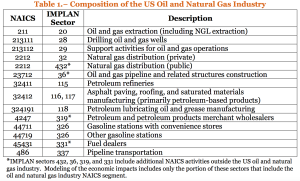
In the table footnote you can see that the API – PwC economic assessment was limited to the oil and gas industry itself, and their results did not include the economic value of the many downstream businesses whose operations are dependent on one or more of the various products delivered by the oil and gas industry (i.e., plastic and synthetic material manufacturers, airlines, trucking, power plants, etc.). If we counted the economic values of these oil and/or gas dependent businesses, then the overall contribution of the oil and gas industry to the U.S. economy would be significantly higher than stated in the API – PwC report. You can get this report at the following link:

http://www.api.org/~/media/Files/Policy/Jobs/Economic_Impacts_ONG_2011.pdf

U.S. oil and gas pipeline infrastructure

Pipeline systems are a key element of the oil and gas industry infrastructure, enabling timely and efficient transportation of the following products:

Crude oil
Petroleum products from crude oil and other liquids processed at refineries, including transportation fuels, fuel oils for heating and electricity generation, asphalt and road oil, and various feedstocks for making chemicals, plastics, and synthetic materials
Hydrocarbon gas liquids (HGL), including natural gas liquids (paraffins or alkanes) and olefins (alkenes) produced by natural gas processing plants, fractionators, crude oil refineries, and condensate splitters, but excluding liquefied natural gas (LNG) and aromatics
Natural gas

The U.S. has over 200,000 miles of liquids pipelines that, in 2014, transported 16.2 billion barrels of crude oil, petroleum products and HGL. More than 17,000 miles of liquid pipelines were added to the network in the five-year period from 2010 thru 2014. The U.S. has over 300,000 miles of interstate and intrastate natural gas transmission pipelines. That’s adds up to more than a half million miles of major oil and gas pipelines in the U.S.

Most pipelines are installed underground, with pumping / compressor stations at grade level. The Trans-Alaska pipeline system is a notable exception, with its above-grade pipeline in permafrost regions.

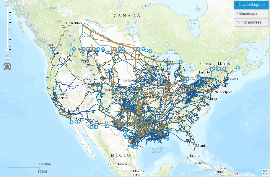
The U.S. Energy Information Agency (EIA) maintains the U.S. Energy Mapping System, which is a geographic information system (GIS) that can display a great deal of energy infrastructure information. The user can select the map area to be viewed, the map style, and the data to be displayed on the map. Once you’ve created the map of your choice, you can zoom and scroll to explore map details. You can access the U.S. Energy Mapping System at the following link:

https://www.eia.gov/state/maps.cfm

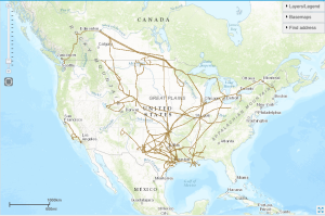
The following maps prepared using the U.S. Energy Mapping System show the distribution of oil and gas pipeline systems in the U.S. (except Alaska & Hawaii) and Canada. The source of pipeline mileage data is the Pipeline and Hazardous Material Safety Administration (PHMSA). The source of liquid capacity data is the Association of Oil Pipe Lines (AOPL).

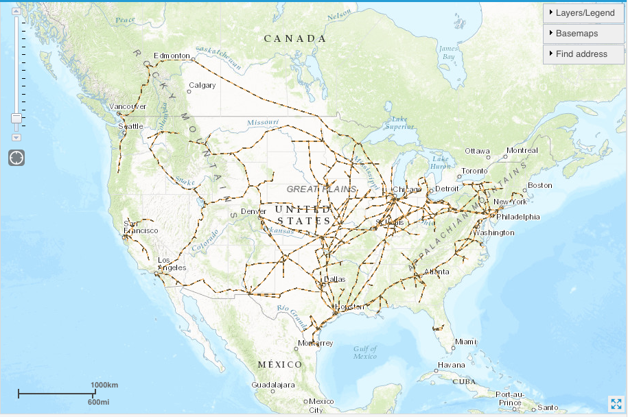
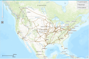
Crude oil pipelines:

73,300 miles of interstate and intrastate pipelines in 2015 (PHMSA)
Delivered 9.3 billion barrels (bbl) of crude oil nationwide in 2014 (AOPL)

Petroleum product pipelines:

62,588 miles of interstate and intrastate pipelines in 2015 (PHMSA)
The petroleum product pipelines and the HGL pipelines together delivered 6.9 billion barrels (bbl) of products nationwide in 2014 (AOPL).

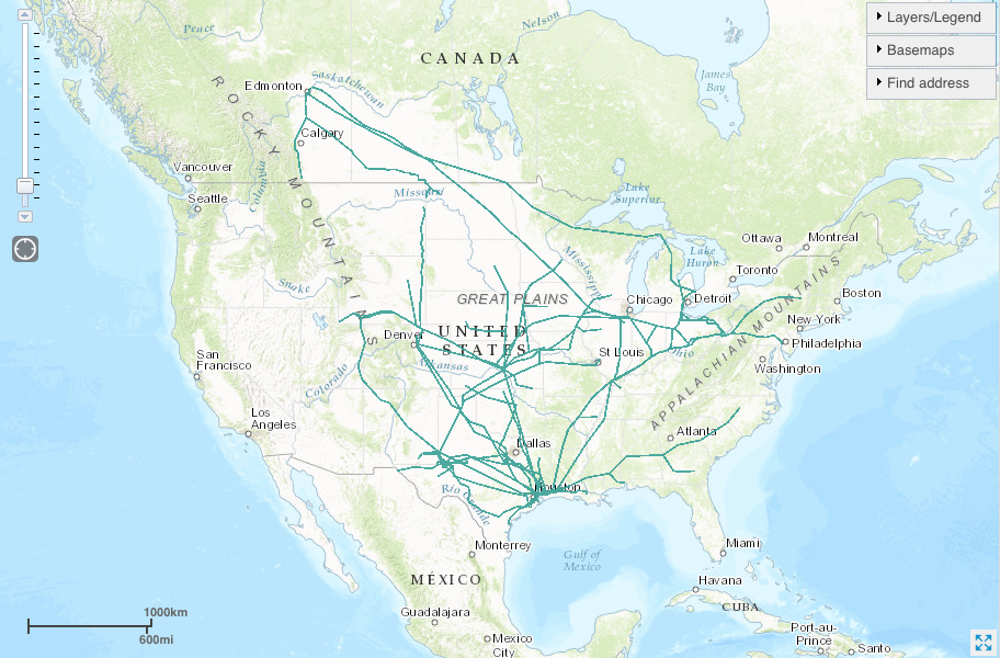
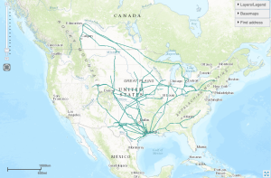
HGL (natural gas liquids) pipelines:

67,577 miles of interstate and intrastate pipelines in 2015 (PHMSA)

Natural gas pipelines:

2,509,000 total miles of natural gas pipelines in 2015 (PHMSA)
- 301,242 miles of interstate and intrastate transmission pipelines
- 1.28 million miles of gas distribution main lines (smaller than the transmission pipelines)
- 913,085 miles of gas distribution service lines
- 17,727 miles of gathering mains that collect gas from wells and move it through a series of compression stages to the main transmission pipelines
Natural gas transmission pipeline capacity was approximately 443 billion cubic feet per day in 2011 (QER 1.1)

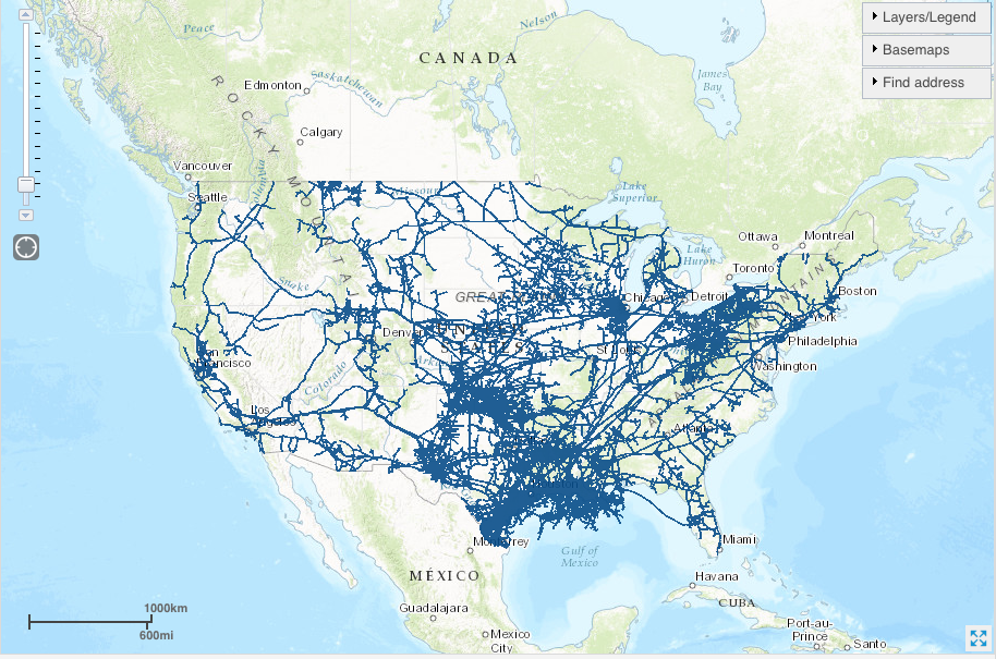
All of the above maps combined, including international border crossings:

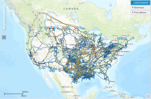
The high density of pipeline systems in many parts of the nation is evident in the last map. On the EIA’s U.S. Energy Mapping System website, you can recreate and explore any of the above maps.

Pipeline safety

The Department of Transportation’s (DOT) Pipeline and Hazardous Material Safety Administration (PHMSA), acting through the Office of Pipeline Safety (OPS), administers the DOT national regulatory program to assure the safe transportation of natural gas, petroleum, and other hazardous materials by pipeline.

PHMSA has collected pipeline incident reports since 1970. PHMSA defines “significant incidents” as any of the following conditions that originate within the pipeline system (but not initiated by a nearby external event that affects the pipeline system).

Fatality or injury requiring in-patient hospitalization
$50,000 or more in total costs, measured in 1984 dollars
Highly volatile liquid releases of 5 barrels (210 gallons) or more, or other liquid releases of 50 barrels (2,100 gallons) or more
Liquid releases resulting in an unintentional fire or explosion

PHMSA data are available at the following link:

http://www.phmsa.dot.gov/pipeline/library/data-stats

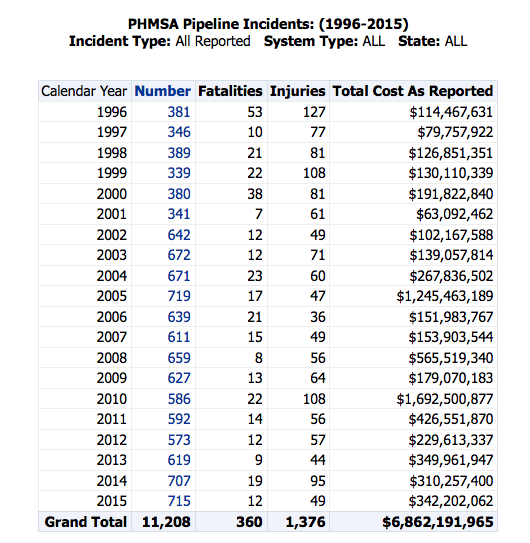
A summary of all reported pipeline incidents over the past 20 years is presented in the following PHMSA table.

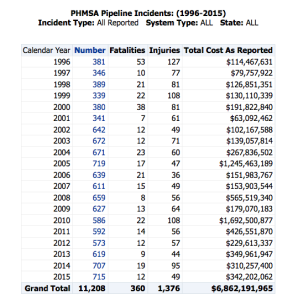
The 20-year averages (1996 – 2015) are:

Incidents: 560
Fatalities: 18
Injuries: 69
Total cost: $343,109,598

The latest data for 2016 (possibly not final) are:

Incidents: 620
Fatalities: 17
Injuries: 82
Total cost: $275,341,057

Clearly, the oil and gas pipeline business is quite hazardous, and the economic cost of pipeline incidents is very high, even in an average year. Since the mid-1990s, the number of incidents per year has almost doubled (367 average for 1996 – 2000 vs. 641 average for 2011 – 2015) as has the total cost per year ($128.4 million average for 1996 – 2000 vs. $331.6 million average for 2011 – 2015).

In June 2015, Jonathan Thompson posted the article, “Mapping 7 Million Gallons of Crude Oil Spills,” on the High Country News website, at the following link:

http://www.hcn.org/articles/spilling-oil-santa-barbara/print_view

In this article, High Country News mapped the last five years of PHMSA data, which included more than 1,000 crude oil pipeline leaks and ruptures. Key points made in the High Country News article are

Over the five-year period, 168,000 barrels (more than 7 million gallons) of crude oil were spilled as a result of reported incidents. That’s an average of about 1.4 million gallons (33,600 barrels) per year leaking or spilled from 73,300 miles of crude oil pipelines that delivered 3 billion barrels of oil annually in 2014. That annualized amount of leakage also is equivalent to the amount of oil carried in about 47 DOT-111 rail cars.
Commonly reported causes included poor material condition (corrosion, bad seals), weather (heavy rains, lightning), and human error (valves being left open, people puncturing pipelines while digging).
Many of the spills were small, releasing less than 10 barrels (420 gallons) of oil, but a few were much larger. For example, a 2013 lightning strike on a North Dakota pipeline caused a 20,000-barrel (840,000 gallon) leak.

Cleanup after these spills and leaks is included in the PHMSA total cost data.

Aging infrastructure

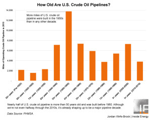
Is August 2014, Jordan Wirfs-Brock posted the article, “Half Century Old Pipelines Carry Oil and Gas Load,” on the Inside Energy (IE) website at the following link:

http://insideenergy.org/2014/08/01/half-century-old-pipelines-carry-oil-and-gas-load/

Using PHMSA data, the author mapped the age of the U.S. pipeline infrastructure and determined that, “About forty-five percent of U.S. crude oil pipeline is more than fifty years old.” The following chart shows the age distribution of U.S. crude oil pipelines.

In April 2015 Administration issued the First Installment of the Quadrennial Energy Review (QER 1.1). This report included the following chart showing the age distribution of U.S. natural gas transmission and gathering pipelines. It looks like more than 50% of these natural gas pipelines are more than 50 years old.

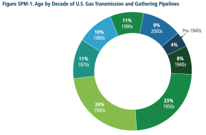
Source: QER 1.1 Summary

The high percentage of older pipeline systems places the overall integrity, reliability and safety of the critical national pipeline infrastructure at risk.

Pipeline modernization

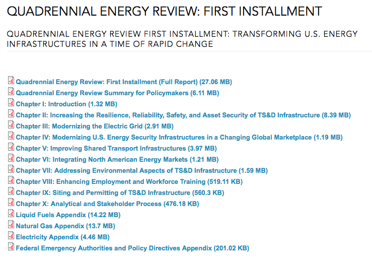
In a previous post, I described the Quadrennial Energy Review (QER) initiated by the Obama Administration in January 2014. The first QER report, QER 1.1, released in April 2015, provides a good overview of issues related to oil and gas pipeline system risks and opportunities to modernize this critical infrastructure.

One positive step was taken on 16 April 2015 by the Federal Energy Regulatory Commission (FERC) when it announced a new policy, Cost Recovery Mechanisms for Modernization of Natural Gas Facilities. This policy sets conditions for interstate natural gas pipeline operators to recover certain safety, environmental, or reliability capital expenditures made to modernize pipeline system infrastructure.

Given the scale of the national oil and gas pipeline infrastructure, and the age of significant portions of that infrastructure, it will take decades of investment to implement system-wide modernization. The political climate, economic climate, and maybe the stars need to be in alignment for this enormous, long-term modernization effort to deliver the needed results.

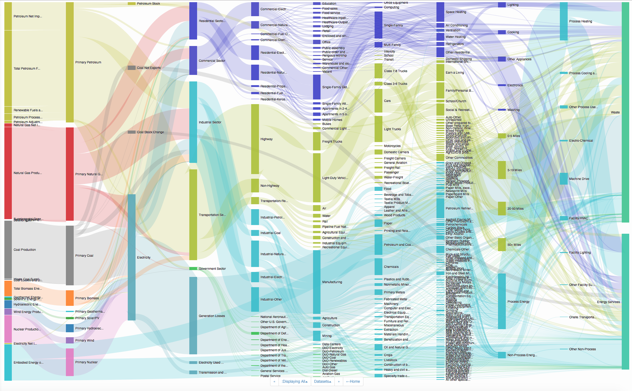
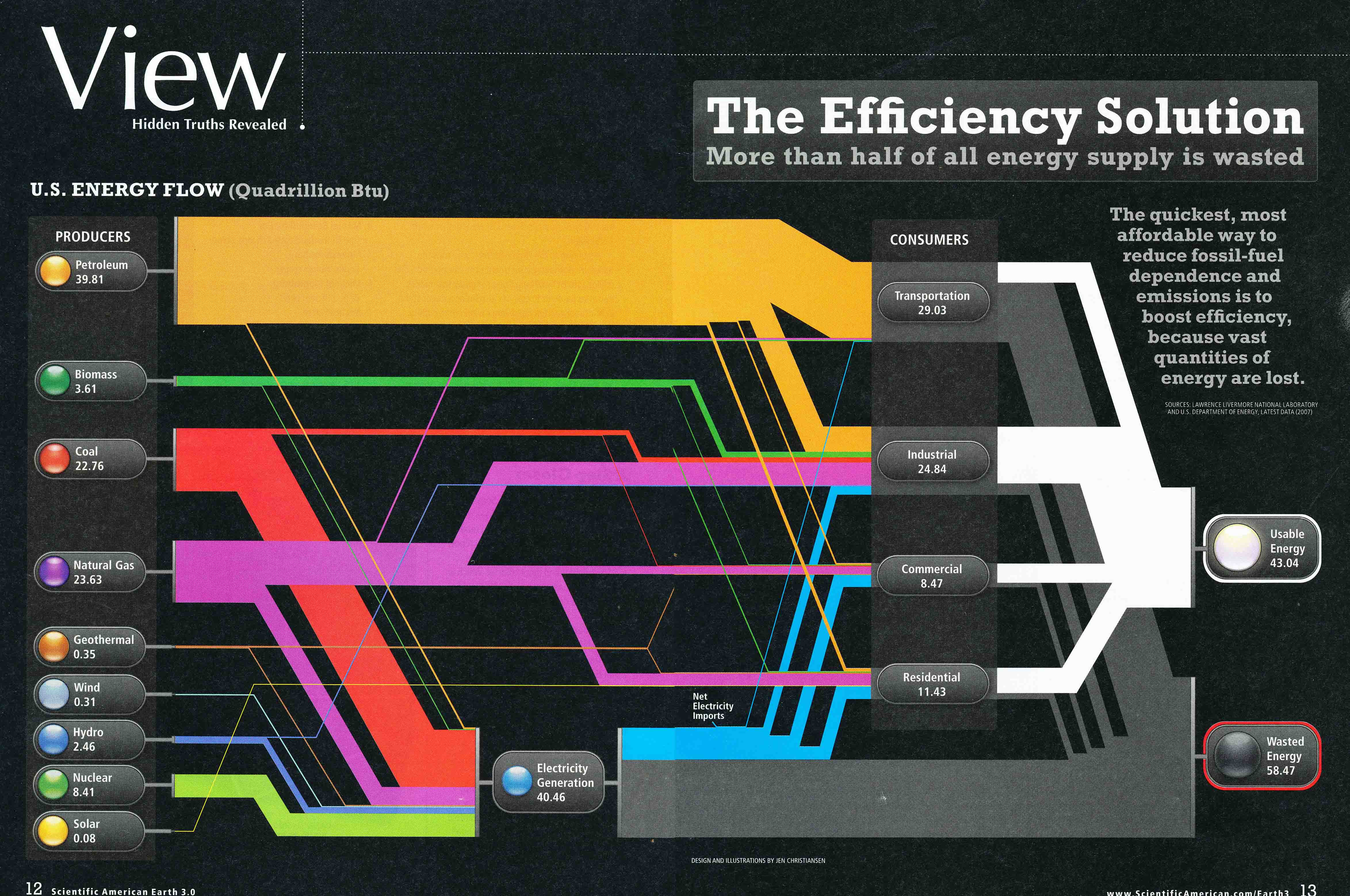
Quadrennial Energy Review

January 19, 2017All Posts, Energy, Oil & gas, Power Generating Technology - Alternate, Power Generating Technology - Fossil, Power Generating Technology - Nuclear, Power Storage Technology, TransportationQER 1.1, QER 1.2, Quadrennial Energy ReviewDrummer

Peter Lobner

On 9 January 2014 the Administration launched a “Quadrennial Energy Review” (QER) to examine “how to modernize the Nation’s energy infrastructure to promote economic competitiveness, energy security, and environmental responsibility…” You can read the Presidential Memorandum establishing the QER at the following link:

https://www.whitehouse.gov/the-press-office/2014/01/09/presidential-memorandum-establishing-quadrennial-energy-review

You can get a good overview of the goals of the QER in a brief factsheet at the following link:

https://www.whitehouse.gov/the-press-office/2015/04/21/fact-sheet-administration-announces-new-agenda-modernize-energy-infrastr

On April 21, 2015, the QER Task Force released the “first installment” of the QER report entitled “Energy Transmission, Storage, and Distribution Infrastructure.” The Task Force announcement stated:

“The first installment (QER 1.1) examines how to modernize our Nation’s energy infrastructure to promote economic competitiveness, energy security, and environmental responsibility, and is focused on energy transmission, storage, and distribution (TS&D), the networks of pipelines, wires, storage, waterways, railroads, and other facilities that form the backbone of our energy system.”

The complete QER 1.1 report or individual chapters are available at the following link:

https://energy.gov/epsa/quadrennial-energy-review-first-installment

QER 1.1 contents are listed below:

On January 6, 2017, the QER Task Force released the “second installment” of the QER report entitled “Transforming the Nation’s Electricity System.” The Task Force announcement stated:

“The second installment (QER 1.2) finds the electricity system is a critical and essential national asset, and it is a strategic imperative to protect and enhance the value of the electricity system through modernization and transformation. QER 1.2 analyzes trends and issues confronting the Nation’s electricity sector out to 2040, examining the entire electricity system from generation to end use, and within the context of three overarching national goals: (1) enhance economic competitiveness; (2) promote environmental responsibility; and (3) provide for the Nation’s security.

The report provides 76 recommendations that seek to enable the modernization and transformation of the electricity system. Undertaken in conjunction with state and local governments, policymakers, industry, and other stakeholders, the recommendations provide the building blocks for longer-term, planned changes and activities.”

The complete QER 1.2 report or individual chapters are available at the following link:

https://energy.gov/epsa/quadrennial-energy-review-second-installment

QER 1.2 contents are listed below:

I hope you take time to explore the QERs. I think the Task Force has collected a great deal of actionable information in the two reports. Converting this information into concrete actions will be a matter for the next Administration.

NuScale Submits First Ever Design Certification Application (DCA) for a Small Modular Reactor (SMR)

January 18, 2017All Posts, Power Generating Technology - NuclearDCA, Design Certification Application, NRC, Nuclear Regulatory Commission, NuScale, NuScale Power Modules, small modular reactor, SMRDrummer

Peter Lobner

For all the talk about SMRs over the past two decades or more, there have been no SMR license applications submitted to the U.S. Nuclear Regulatory Commission (NRC) until now. On 31 December 2016, NuScale Power, Portland, OR made the first ever request to the NRC to initiate a licensing review of an SMR. On 12 January 2017, NuScale made the formal submittal to NRC of all the required DCA documents for an SMR power plant comprised of 12 individual NuScale Power Modules^TM.

An NPM is a small pressurized water reactor (PWR) with an integrated primary system and many passive features for normal modes of operation and for safe shutdown in response to abnormal or accident conditions. NuScale claims that the passive safety features enable shutdown and self-cooling with no operator action, no AC or DC power, and no external water.

You’ll find a good 2013 overview of the NuScale Power Module^TM on the IAEA’s (International Atomic Energy Agency’s) ARIS (Advanced Reactor Information System) website at the following link:

https://aris.iaea.org/sites/..%5CPDF%5CNuScale.pdf

More information is available on the NuScale Power website at the following link:

http://www.nuscalepower.com

The basic, factory-manufactured NPM is rated at 160 MWt, which could deliver about 45 MWe. A power plant with 12 NPMs would have a combined output of 1,920 MWt and about 540 MWe. A single NPM is shown below.

Source: NuScale Power

NuScale Power anticipates a 42-month licensing process as outlined in the following chart. If this schedule can be achieved, then the NRC could issue a Design Certification (DC) as soon as July 2020. At that time, the standard design of a modular NuScale power plant with up to 12 NPMs will have NRC approval independent of an application to construct or operate a specific plant. A design certification is valid for 15 years from the date of issuance and can be renewed.

Source: NuScale Power

A license application for an actual plant will focus on site-specific issues and should not need to re-open issues already covered in the NRC’s DC review. This greatly de-risks construction of a new nuclear power plant based on the NPM standard design approved in the DC. NuScale forecasts that the first NPM could go into operation as soon as 2024.