Category Archives: Physics

Where in the Periodic Table Will We Put Element 119?

Peter Lobner

The first periodic table of elements

In 1869, Russian chemist Dimitri Mendeleev proposed the first modern periodic table of elements, in which he arranged the 60 known elements in order of their increasing atomic masses (average mass, considering relative abundance of isotopes in naturally-occurring elements), with elements organized into groups based their similar properties. Mendeleev observed that certain properties recur at regular intervals in the periodic table, thereby defining the groupings of elements.

Mendeleev stamp 
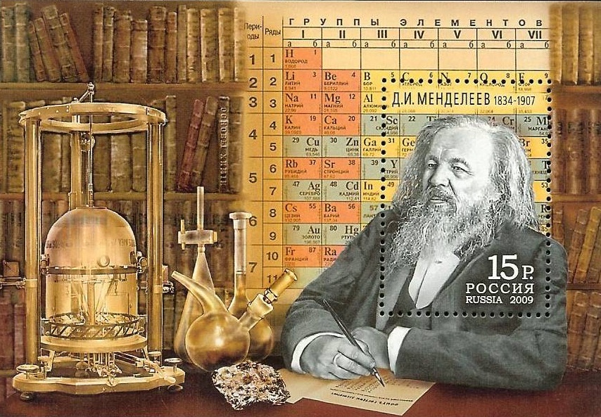
Source: http://we-are-star-stuff.tumblr.com

This first version of the periodic table is compared to the modern periodic table in the following diagram prepared by SIPSAWIYA.COM. Mendeleev’s periodic table consisted of Groups I to VIII in the modern periodic table.

Mendeleev_sipsawiyagif

The gaps represent undiscovered elements predicted by Mendeleev’s periodic table, for example, Gallium (atomic mass 69.7) and Germanium (atomic mass 72.6) . You can read more about Mendeleev’s periodic table at the following link:

http://www.sipsawiya.com/2015/07/history-of-periodic-table.html

German chemist Lothar Meyer was competing with Mendeleev to publish the first periodic table. The general consensus is that Mendeleev, not Meyer, was the true inventor of the periodic table because of the accuracy and detail of Mendeleev’s work.

Element mendelevium (101) was named in honor of Dimitri Mendeleev.

Evolution of the Modern Periodic Table of Elements

The modern periodic table organizes elements according to their atomic numbers (number of protons in the nucleus) into 7 periods (vertical) and 18 groups (horizontal). The version shown below, in the International Union of Pure and Applied Chemistry (IUPAC) format, accounts for elements up to atomic number 118 and color-codes 10 different chemical series.

PeriodicTableMeltingPoint

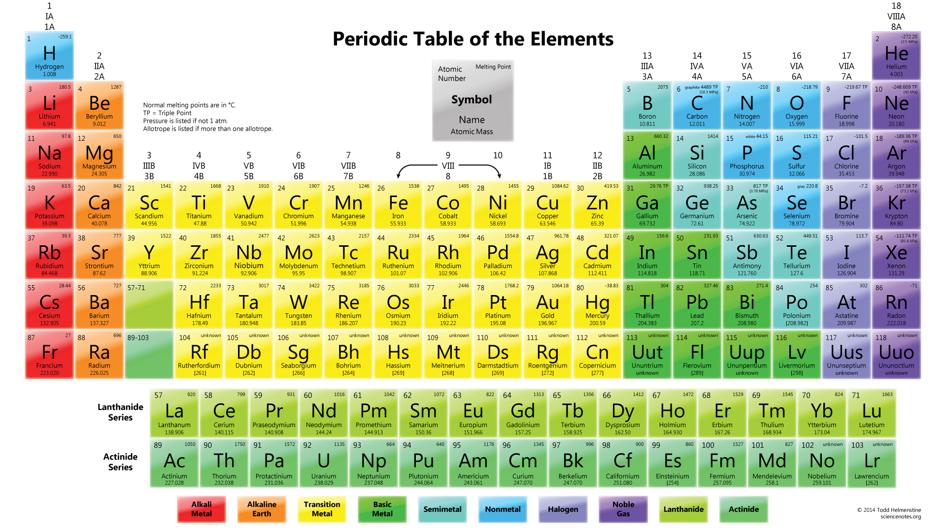
Source: http://sciencenotes.org/printable-periodic-table/

Hundreds of versions of the periodic table of elements have existed since Mendeleev’s first version. You can view a great many of these at The Internet Database of Periodic Tables curated by Dr. Mark R. Leach and presented at the following link:

http://www.meta-synthesis.com/webbook/35_pt/pt_database.php?Button=All

Glenn T. Seaborg (1912 – 1999) is well known for his role in defining the structure of the modern periodic table. His key contributions to periodic table structure include:

  • In 1944, Seaborg formulated the ‘actinide concept’ of heavy element electron structure, which predicted that the actinides, including the first 11 transuranium elements, would form a transition series analogous to the rare earth series of lanthanide elements. The actinide concept showed how the transuranium elements fit into the periodic table.
  • Between 1944 and 1958, Seaborg identified eight transuranium elements: americium (95), curium (96), berkelium (97), californium (98), einsteinium (99), fermium (100), mendelevium (101), and nobelium (102).

Element seaborgium (106) was named in honor of Glenn T. Seaborg.  Check out details Glenn T. Seaborg’s work on transuranium elements at the following link:

http://www.osti.gov/accomplishments/seaborg.html

Four newly-discovered and verified elements

On 30 December 2015, IUPAC announced the verification of the discoveries of the following four new elements: 113, 115, 117 and 118.

  • Credit for the discovery of element 113  was given to a team of scientists from the Riken institute in Japan.
  • Credit for discovery of elements 115 , 117 and 118 was given to a Russian-American team of scientists at the Joint Institute for Nuclear Research in Dubna and Lawrence Livermore National Laboratory in California.

These four elements complete the 7th period of the periodic table of elements. The current table is now full.

You can read this IUPAC announcement at the following link:

http://www.iupac.org/news/news-detail/article/discovery-and-assignment-of-elements-with-atomic-numbers-113-115-117-and-118.html

On 28 November 2016, the IUPAC approved the names and symbols for these four new elements: nihonium (Nh), moscovium (Mc), tennessine (Ts), and oganesson (Og), respectively for element 113, 115, 117, and 118.  Nihonium was the first element named in Asia.

Dealing with super-heavy elements beyond element 118

The number of physically possible elements is unknown.

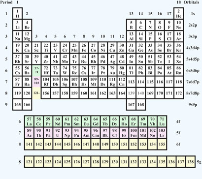
In 1969, Glenn T. Seaborg proposed the following extended periodic table to account for undiscovered elements from atomic number 110 to 173, including the  “super-actinide” series of elements (atomic numbers 121 to 155).

Glenn Seaborg 1969 extended periodic table copy R1Source: W. Nebergal, et al., General Chemistry, 4th ed., pp 668 – 670, D.C. heath Co, Massachusetts, 1972

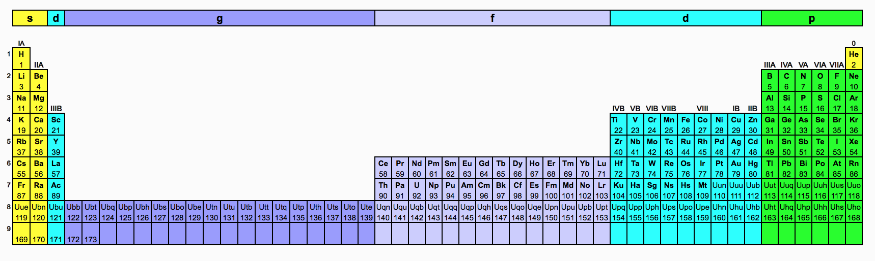
In 2010, Finnish chemist Pekka Pyykkö at the University of Helsinki proposed an extended periodic table with 54 predicted elements. The extension, shown below, is based on a computational model that predicts the order in which the electron orbital shells will fill up, and, therefore, the periodic table positions of elements up to atomic number 172. Pekka Pyykkö says that the value of the work is in showing, “how the rules of quantum mechanics and relativity function in determining chemical properties.”

Pyyko 2010 periodic tableSource: Royal Society of Chemistry

You can read more on Pekka Pyykkö’s extended periodic table at the following link:

http://www.rsc.org/Publishing/ChemScience/Volume/2010/11/Extended_elements.asp

You can read more general information on the extended periodic table on Wikipedia at the following link:

https://en.wikipedia.org/wiki/Extended_periodic_table

So where will we place element 119 in the periodic table of elements?

Based on both the Seaborg and Pyykkö extended periodic tables described above, element 119 will be the start of period 8 and it will be an alkali metal. Element 120 will be an alkaline earth. With element 121, we’ll enter the new chemical series of the “super-actinides”.

These are exciting times for scientists attempting to discover new super-heavy elements.

Where does neutronium fit in the periodic table?

Neutronium is a name coined in 1926 by scientist Andreas von Antropoff for a proposed “element of atomic number zero” (i.e., because it has no protons) that he placed at the head of the periodic table. In modern usage, the extremely dense core of a neutron star is referred to as “degenerate neutronium”.

Neutronium also finds many hypothetical applications in modern science fiction. For example, in the 1967 Star Trek episode, The Doomsday Machine, neutronium formed the hull of a giant, autonomous “planet killer”, and was portrayed as being invulnerable to all manner of scans and weapons. Since free neutrons at standard temperature and pressure undergo β decay with a half-life of 10 minutes, 11 seconds, a very small quantity of neutronium could be quite hazardous to your health.

14 January 2019 Update:  2019 marks the 150th anniversary of Dimitri Mendeleev’s periodic table

You’ll find a very good article, “150 years on, the periodic table has more stories than it has elements,” by Elizabeth Quill on the Science News website.  Here’s the link:

https://www.sciencenews.org/article/periodic-table-elements-chemistry-fun-facts-history

18 January 2019 Update:  Possibly the oldest copy of Mendeleev’s periodic table was found at the University of St. Andrews in Scotland

On 17 January 2019, the University of St. Andrews posted a news article stating that a periodic table of the elements dating from 1885 recently was found at the university and is thought to be the oldest in the world.

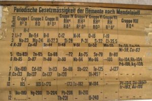
The 1885 periodic table.  Source: University of St. Andrews

You can read the University of St. Andrews news posting here:

https://news.st-andrews.ac.uk/archive/worlds-oldest-periodic-table-chart-found-in-st-andrews/

Just What are Those U.S. Scientists Doing in the Antarctic and the Southern Ocean?

Peter Lobner

The National Academies Press (NAP) recently published the report, “A Strategic Vision for NSF Investments in Antarctic and Southern Ocean Research”, which you can download for free at the following link if you have established a MyNAP account:

http://www.nap.edu/catalog/21741/a-strategic-vision-for-nsf-investments-in-antarctic-and-southern-ocean-research

Print Source: NAP

NSF states that research on the Southern Ocean and the Antarctic ice sheets is becoming increasingly urgent not only for understanding the future of the region but also its interconnections with and impacts on many other parts of the globe. The research priorities for the next decade, as recommended by the Committee on the Development of a Strategic Vision for the U.S. Antarctic Program; Polar Research Board; Division on Earth and Life Studies; National Academies of Sciences, Engineering, and Medicine, are summarized below:

  • Core Program: Investigator-driven basic research across a broad range of disciplines
    • NSF gives the following rationale: “…it is impossible to predict where the next major breakthroughs or advances will happen. Thus to ensure that the nation is well positioned to take advantage of such breakthroughs, it is important to be engaged in all core areas of scientific research.”
      • NSF notes, “…discoveries are often made by single or small groups of PIs thinking outside the box, or with a crazy new idea, or even just making the first observations from a new place.”
    • Examples of basic research that have led to important findings include:
      • Ross Sea food chain is affected by a high abundance of predator species (whales, penguins and toothfish) all competing for the same limited resource: krill. Decline or recovery of one predator population can be seen in an inverse effect on the other predator populations.  This food chain response is not seen in other areas of the Antarctic ice shelf where predator populations are lower, allowing a larger krill population that adequately supports all predators.
      • Basic research into “curious” very-low frequency (VLF) radio emissions produced by lightning discharges led to a larger program (with a 21.2-km-long VLF antenna) and ultimately to a better understanding of the behavior of plasma in the magnetosphere.
  • Strategic, Large Research Initiatives –  selection criteria:
    • Primary filter: compelling science – research that has the potential for important, transformative steps forward in understanding and discovery
    • Subsequent filters: potential for societal impact; time-sensitive in nature; readiness / feasibility; and key area for U.S. and NSF leadership.
    • Additional factors: partnership potential; impact on program balance; potential to help bridge existing disciplinary divides
  • Strategic, Large Research Initiative – recommendations::
    • Priority I: The Changing Antarctic Ice Sheets Initiative to determine how fast and by how much will sea level rise?
      • A multidisciplinary initiative to understand why the Antarctic ice sheets is changing now and how they will change in the future.
      • Will use multiple records of past ice sheet change to understand rates and processes.
    • Priority II: How do Antarctic biota evolve and adapt to the changing environment?
      • Decoding the genomic (DNA) and transcriptomic (messenger RNA molecules) bases of biological adaptation and response across Antarctic organisms and ecosystems.
    • Priority III: How did the universe begin and what are the underlying physical laws that govern its evolution and ultimate fate?
      • A next-generation cosmic microwave background (CBM) program that builds on the current successful CMB program using telescopes at the South Pole and the high Atacama Plateau in Chile and possibly will add a new site in the Northern Hemisphere to allow observations of the full sky

You will find detailed descriptions of the Priority I to III strategic programs in the Strategic Vision report.

100th Anniversary of Einstein’s General Theory of Relativity and the Advent of a New Generation of Gravity Wave Detectors

Peter Lobner

One hundred years ago, Albert Einstein presented his General Theory of Relativity in November 1915, at the Prussian Academy of Science. Happy Anniversary, Dr. Einstein!

Today, general relativity is being tested with unprecedented accuracy with a new generation of gravity-wave “telescopes” in the U.S., Italy, Germany, and Japan. All are attempting to directly detect gravity waves, which are the long-predicted quakes in space-time arising from cataclysmic cosmic sources.

The status of four gravity-wave telescopes is summarized below.

USA: Laser Interferometer Gravitational-Wave Observatory (LIGO)

LIGO is a multi-kilometer-scale gravitational wave detector that uses laser interferometry to, hopefully, measure the minute ripples in space-time caused by passing gravitational waves. LIGO consists of two widely separated interferometers within the United States; one in Hanford, WA and the other in Livingston, LA. These facilities are operated in unison to detect gravitational waves. The Livingston and Hanford LIGO sites are shown in the following photos (Hanford above, Livingston below):

ligo-hanford-aerial-02Source LIGO Caltechligo-livingston-aerial-03Source: LIGO Caltech

LIGO is operated by Caltech and MIT and is supported by the National Academy of Sciences. For more information, visit the LIGO website at the following link:

https://ligo.caltech.edu/page/about

Basically, LIGO is similar to the traditional interferometer used in 1887 in the famous Michelson-Morley experiment (https://en.wikipedia.org/wiki/Michelson–Morley_experiment). However, the LIGO interferometer incorporates novel features to greatly increase its sensitivity. The basic arrangement of the interferometer is shown in the following diagram.

LIGO experiment setupSource: LIGO Caltech

Each leg of the interferometer has a physical length of 4 km and is a resonant Fabry-Perot cavity that uses a complex set of mirrors to extend the effective arm length by a factor of 400 to 1,600 km.

On 18 September 2015, the first official “observing run” using LIGO’s advanced detectors began. This “observing run” is planned to last three months. LIGO’s advanced detectors are already three times more sensitive than Initial LIGO was by the end of its observational lifetime in 2007. You can read about this milestone event at the following link:

https://ligo.caltech.edu/news/ligo20150918

You also can find much more information on the LIGO Scientific Collaboration (LSC) at the following link:

http://www.ligo.org

Italy: VIRGO

VIRGO is installed near Pisa, Italy, at the site of the European Gravitational Observatory (http://www.ego-gw.it/public/virgo/virgo.aspx). VIRGO is intended to directly observe gravitational waves using a Michelson interferometer with arms that are 3 km long, with resonant Fabry-Perot cavities that increase the effective arm length by a factor of 50 to 150 km. The initial version of VIRGO operated from 2007 to 2011 and the facility currently is being upgraded with a new, more sensitive detector. VIRGO is expected to return to operation in 2018.

You can find much more information on VIRGO at the following link:

http://www.virgo-gw.eu

Germany: GEO600

GEO600 is installed near Hanover, Germany. It, too, uses a Michelson interferometer with arms that are 600 meters long, with resonant Fabry-Perot cavities that double the effective arm length to 1,200 meters.

You can find much more information on the GEO600 portal at the following link:

http://www.geo600.org

Japan: KAGRA Large-scale Cryogenic Gravitational Wave Telescope

The KAGRA telescope is installed deep underground, in tunnels of Kamioka mine, as shown in the following diagram.

img_abt_lcgtSource: KAGARA

Like the other facilities described previously, KAGRA is a Michelson interferometer with resonant Fabry-Perot cavities. The physical length of each arm is of 3 km (1.9 mi). KAGRA is expected to be in operation in 2018.

You can find much more information on KAGARA at the following links:

http://www.astro.umd.edu/~miller/Compact/lcgt.pdf

and,

http://gwcenter.icrr.u-tokyo.ac.jp/en/

The Magnus Effect and its Broad Applications: From Sports to Ballistics to Dam Busting in WW II

Peter Lobner

The Magnus effect occurs when a moving spherical or cylindrical body has a spin. The observed effect is that the moving, spinning body moves away from the intended direction of travel. The spin alters the airflow around the moving body and, by conservation of momentum, generates the Magnus force. In the case of a flying (thrown) backspinnning round body shown below, the Magnus force is a lift.

Sketch_of_Magnus_effectSource: Wikipedia

The Magnus force is named for German physicist Heinrich Gustav Magnus, who described the effect in 1852. Other scientists had described the effect long before Magnus, notably Isaac Newton (in 1672) and British mathematician and ballistic researcher Benjamin Robins (in 1742), but it was Magnus who got the honor.

We can see the Magnus effect at work in sports and in other applications discussed below.

Baseball

The pitcher can impart a spin in a selected direction to throw a curveball, slider or other pitch. Major League Baseball (MLB) uses a system called PITCHf/x, which is installed in every MLB stadium, to track the speed and trajectory of pitched baseballs. The system calculates two values, BRK and PFX, related to the Magnus effect:

  • BRK is a measure of the amount of bend in the trajectory at its greatest distance from a straight line
  • PFX is a measure of the deflection of the baseball due to the spin and drag forces from the path it would have taken under the influence of gravity alone

You can find more information on PITCHf/x at the following links:

https://en.wikipedia.org/wiki/PITCHf/x

and,

http://www.fangraphs.com/library/misc/pitch-fx/

Golf

A backspin on a golf ball creates a lift, as shown in the diagram above, helping to extend the range of the shot. A topspin has the opposite effect, shortening the ball’s trajectory. A spin about a vertical or diagonal axis results in a slice or hook to the right or left, invariably putting the ball into deep grass or some other course hazard. I have trouble visualizing how a golfer imparts a spin about the ball’s vertical or diagonal axis, but apparently it is a lot easier that you might think.

Extreme basketball

Thanks to Dave Groce, who forwarded the following link to a video that demonstrates how the Magnus effect helped a group in Tasmania sink a basketball from the top of a dam.  I have a feeling that there were a lot more basketballs at the bottom of the dam than are shown in the video.

https://www.youtube.com/watch?v=2OSrvzNW9FE

Ballistics

A spinning bullet will encounter a Magnus force if it yaws slightly in flight (i.e., direction of the central axis of the bullet is slightly different than its direction of flight, or velocity vector) or is shot into a crosswind. The direction of the Magnus force will depend on the direction of yaw or crosswind. A sniper shooting at long range needs to consider the Magnus effect.

WW II Dambusters

As reported on the Bomber Command website (http://www.bombercommandmuseum.ca/damsraid1.html):

 “The Dams Raid was conceived in the brilliant mind of Barnes Wallis, an experienced aircraft designer. Wallis had designed the very successful Wellington bomber that had been operational since the beginning of the war and, in his spare time, he searched for weaknesses in the enemy’s industrial infrastructure. The hydroelectric dams of the highly Ruhr Valley became his focus.

He devised a cylindrical, 9,500 pound weapon that could be dropped at low level while rotating backwards at 500 rpm. Released from a height of 60 feet, about 450 yards from the dam, and at a speed of 230 miles per hour, the weapon would then skip along the water (and over any torpedo nets) until it struck the dam wall, the spinning maintaining the weapon’s stability and slowing it down.

The backward rotation would then cause the cylinder to roll down the dam wall where it would explode at a predetermined depth. The wall would be weakened and the great weight of water would cause the dam to collapse.”

Experiments performed by Wallis demonstrated that the Magnus effect gave aerodynamic lift to the bomb and thereby increased the number of bounces before the bomb either struck the dam or stopped bouncing and sank.

p_damsraid1bSource: Bomber Command Museum

There is much more information on Sir Barnes Wallis and the Dams Raid on the Bomber Command website.

For more information, I also recommend the book, “Dam Busters: The True Story of the Inventors and Airmen Who Led the Devastating Raid to Smash the German Dams in 1943,” by James Holland, published by Grove Press, New York, and available in paperback in 2014, ISBN-13: 978-0802122780.

Kurzgesagt Explains the Fermi Paradox: Where are all the aliens?

Peter Lobner, updated 17 November 2022

Kurzgesagt (German for “in a nutshell“) is a Munich-based design studio with a distinctive perspective on design and animation in the fields of education, science and commerce.  For background information on Kurzgesagt, visit their website here: https://kurzgesagt.org/agency/

You’ll find their YouTube channel with a library of briefings at the following link: https://www.youtube.com/channel/UCsXVk37bltHxD1rDPwtNM8Q

From here you can navigate to many intriguing and entertaining animated briefings.  Four Kurzgesagt briefings address the following questions regarding extraterrestrial life:

“The universe is unbelievably big – trillions of stars and even more planets. Soo… there just has to be life out there, right? But where is it? Why don’t we see any aliens? Where are they? And more importantly, what does this tell us about our own fate in this gigantic and scary universe?”

I hope you’ll enjoy these Kurzgesagt briefings:

The Fermi Paradox — Where Are All The Aliens? Part 1:  https://www.youtube.com/watch?v=sNhhvQGsMEc

The Fermi Paradox — Where Are All The Aliens? Part 2:  https://www.youtube.com/watch?v=1fQkVqno-uI

The Great Filter:  Why Alien Life Would be our Doom:  https://www.youtube.com/watch?v=UjtOGPJ0URM

What Do Alien Civilizations Look Like? The Kardashev Scale:  https://www.youtube.com/watch?v=rhFK5_Nx9xY

Aliens under the Ice – Life on Rogue Planets:  https://www.youtube.com/watch?v=M7CkdB5z9PY

For more information

LightSail to Demonstrate the Feasibility of Solar Sail Technology for Future Spacecraft Propulsion

Peter Lobner

Light exerts a measurable pressure on solid objects. This was demonstrated in 1899 in an experiment conducted by Russian scientist Pyotr Nikolayevich Lebedev. This experiment also demonstrated that the pressure of light is twice as great on a reflective surface than on an absorbent surface. This is the basis for the solar sail concept for spacecraft propulsion.

Solar sailing  Source:  Planetary Society

The Japanese IKAROS (Interplanetary Kite-craft Accelerated by Radiation Of the Sun) spacecraft launched on 20 May 2010 is the world’s first spacecraft to use solar sailing as its main propulsion. The square solar sail measured 14.14 meters (46.4 feet) along its edge, with a total area of 200 square meters (2,153 square feet). Thin-film solar cells in the sail provide electric power for spacecraft systems. IKAROS was launched as a secondary payload in conjunction with the Japanese Venus Climate Orbiter. The Japanese Aerospace Exploration Agency (JAXA) claims that acceleration and attitude control of IKAROS were demonstrated during the spacecraft’s flight toward Venus. The total velocity effect over the six-month flight to Venus was reported to be 100 m/s. IKAROS continued into solar orbit while its companion spacecraft entered orbit around Venus.

The Planetary Society conceived and is executing a crowd-funded project called LightSail to continue demonstrating the feasibility of solar sail technology. You can read more at their website:

http://sail.planetary.org

Packaged into a compact 3-unit “CubeSat” (about the size of a loaf of bread) for launch, the Planetary Society’s first LightSail spacecraft, LightSail A, hitched a ride into orbit on an Air Force Atlas V booster on 20 May 2015. The primary purpose of this first mission is to demonstrate that LightSail can deploy its 32 square meter (344 square foot) reflective Mylar solar sail properly in low Earth orbit.  Following launch and orbital checkout, the sail is expected to be deployed 28 days after launch. Thereafter, atmospheric drag will cause the orbit to decay.

LightSail A spacecraft Source: Planetary Society

You can read more about the first mission at the following link:

http://www.wired.com/2015/05/blasting-off-today-satellite-sails-sunbeams/?mbid=social_twitter&utm_source=howtogeek&utm_medium=email&utm_campaign=newsletter

In a second mission planned for 2016, LightSail B will be deployed into a higher orbit with the primary purpose of demonstrating propulsion and maneuverability. LightSail B will be similar to LightSail A, with the addition of a reaction wheel that will be used to control the orientation of the spacecraft relative to the Sun. This feature should allow the spacecraft to tack obliquely relative to the photon stream from the Sun, enabling orbital altitude and/or inclination to be changed.

You can find more information on solar sail physics and use of this technology at the following link:

http://en.wikipedia.org/wiki/Solar_sail

 29 May 2015, Update 1:

After launch, the LightSail A spacecraft’s computer was disabled by a software problem and the spacecraft lost communications with Earth.  Reset commands have failed to reboot the computer.  The computer and communications problems occurred before the solar sail was scheduled to be deployed.

31 May 2015, Update 2:

The LightSail A computer successfully rebooted and communications between the spacecraft and the ground station have been restored.  The plan is for ground controllers to install a software fix, and then continue the mission.

9 June 2015, Update 3:

The Planetary Society announced that the LightSail A spacecraft successfully completed its primary objective of deploying a solar sail in low-Earth orbit.

20150609_ls-a-sails-out_f840  Source: Planetary Society

Read their detailed announcement at the following link:

http://www.planetary.org/blogs/jason-davis/2015/20150609-lightsail-test-mission-success.html

CERN Announces Large Hadron Collider (LHC) Return to Operation

Peter Lobner

After a two-year shutdown for modifications that are expected to nearly double the maximum energy of LHC to 13 TeV, CERN has completed a long re-test process and restored LHC to operation. You can read about the restart process at the following link:

http://home.web.cern.ch/about/updates/2014/06/cern-announces-lhc-restart-schedule

image   Source: CERN

Re-start was delayed by an intermittent short circuit that had to be resolved after the superconducting machine had already been cooled down. Maintenance and repair is time-consuming when a superconducting component or system is involved, since the equipment must be warmed up before it can be serviced, and then cooled down again to 1.9 degrees Celsius before LHC operation can resume.

With the LHC back in operation, the search for more Higgs Bosons and signs of supersymmetry continues. Read more about LHC operations at the following link:

http://www.cnet.com/news/after-refit-lhc-accelerator-resumes-hunt-for-new-higgs/

You also might want to review Maria Spiropulo’s 27 August 2014 Lyncean presentation: “The Future of the Higgs Boson.” You can find this presentation in the Past Meetings section of this Lyncean website.

History of the DOE National Laboratories

Peter Lobner

Many at SAIC worked at or for one or more DOE national laboratories at some point in their careers.   The following link to the DOE Office of Scientific & Technical Information (OSTI) web site provides links to other web sites with historical information on the various national labs.

http://www.osti.gov/accomplishments/nuggets/historynatlabs.html

For example, on this OSTI web page, you can select the Idaho National Laboratory link, and a pop-up menu will display the available documents.  If you select, “Proving the Principle: A History of the Idaho Engineering and Environmental Laboratory, 1949 – 1999,” this will take you to an INL web site that includes a 25 chapter history + a 2000 – 2010 addendum, all organized for chapter-by-chapter web access.

I hope you find some something of interest via the OSTI website.

Scientists Used Natural Cosmic Radiation to Peer Inside Fukushima’s Mangled Reactor

Peter Lobner, updated 4 March 2023

Introduction

A muon is an unstable elementary subatomic particle in the same class as an electron (they’re both leptons), but with a much greater mass (207 times greater).  A useful property of muons is that they can penetrate matter much further than X-rays with the added benefit of causing essentially zero damage to the matter it passes through. Muons scatter and lose energy as they pass through matter, slowing down and eventually decaying, typically into three particles: an electron and two types of neutrinos. The higher the average density of the matter encountered along the muon’s flight path, the more quickly the muon slows down.

Muons are created by the interaction of high-energy cosmic rays with the upper regions of Earth’s atmosphere and they account for much of the cosmic radiation that reaches the Earth’s surface. This means that the existing flux of muon radiation at the Earth’s surface (about 10,000 muons/square meter/sec) is a free resource for clever researchers.

Muon tomography uses this free muon flux and the muon’s characteristic of slowing down more quickly in denser matter to create a density map of the field-of-view available to a muon detector.  There are two types of muon imaging, transmission and scattering. The differences are addressed in LA-UR-15-24802, listed below. In both types of muon imaging, denser objects and structures in the detectors field of view appear as shadows (muon shadows) that are darker (fewer muons getting thru to the detectors) than less dense areas.

Muon tomography at the Fukushima Nuclear Power Plant

Tokyo Electric Power Company (TEPCO) supported the use of muon tomography at the Fukushima Nuclear Power Plant to help determine what damage was done to the reactor cores at Units 1, 2 and 3 during the 11 March 2011 accident, which was precipitated by a 9.0 magnitude earthquake followed by a 15-meter (49.2-ft) tsunami.

A 2013 muon tomography feasibility study (Hauro Miyadera, et al.) reported: “Muon scattering imaging has high sensitivity for detecting uranium fuel and debris even through thick concrete walls and a reactor pressure vessel. Technical demonstrations using a reactor mockup, a detector radiation test at Fukushima Daiichi, and simulation studies have been carried out. These studies establish feasibility for the reactor imaging. A few months of measurement will reveal the spatial distribution of the reactor fuel.”

At Reactor #1, two 22 ton (20 metric ton), 21-foot by 21-foot (6.4 m by 6.4 m) muon detectors were installed and used to collect data over periods of months to develop high-resolution images of the damaged reactor core and surrounding areas. Placement of the muon detectors and the general scan geometry is shown in the following diagram.

 
Fukushima muon tomography setup 

Source: LA-UR-12-20494

Reactor #1 muon scan results

In March 2015, TEPCO announced that its muon tomography scanning efforts at Fukushima were successful, and confirmed that the nuclear plant’s Reactor #1 suffered a complete meltdown. The muon scans showed no corium (i.e., the lava-like product of a reactor core meltdown containing the melted nuclear fuel, fission products, control rods, and structural materials) remained in the reactor pressure vessel (RPV). The muon scans did not show the distribution of the corium that flowed out of the bottom of the reactor vessel into the primary containment vessel (PCV).

Muon tomography scan of Reactor #1. The corium, if present in the 
RPV, should have been visible as a dark shadow inside the RPV. 
Source: TEPCO via ExtremeTech (2015)
Muon tomography scan of Reactor #1, focusing on the RPV. 
Source: TEPCO via ExtremeTech (2015)

Reactor #2 muon scan results

World Nuclear News (WNN) reported (2016 & 2017), “TEPCO said analysis of muon examinations of the fuel debris shows that most of the fuel has melted and dropped from its original position within the core (and resolidified)…..Measurements taken between March and July 2016 at unit 2 showed high-density materials, considered to be fuel debris, in the lower area of the RPV.”

A muon tomography image of Reactor #2. 
Source: TEPCO via WNN (2016)

Reactor #3 muon scan results

In 2017, WNN reported, “Some of the fuel in the damaged unit 3 of the Fukushima Daiichi plant has melted and dropped into the primary containment vessel, initial results from using a muon detection system indicate. Part of the fuel, however, is believed to remain in the reactor pressure vessel.”

Muon tomography image of Reactor #3. 
Source: TEPCO via WNN (2017)

Summary of fuel debris status at Fukushima 

Based on the results of the muon tomography program and other means of investigation, TEPCO created the following graphic summary showing the estimated distribution of core and containment vessel fuel debris in Fukushima Units 1, 2 & 3.

Source: TEPCO

For more information