Peter Lobner
My 31 January 2015 post, “Flow Cell Battery Technology Being Tested as an Automotive Power Source,” addressed flow cell battery (also known as redox flow cell battery) technology being applied by the Swiss firm nanoFlowcell AG for use in automotive all-electric power plants. The operating principles of their nanoFlowcell® battery are discussed here:
http://emagazine.nanoflowcell.com/technology/the-redox-principle/
This flow cell battery doesn’t use rare or hard-to-recycle raw materials and is refueled by adding “bi-ION” aqueous electrolytes that are “neither toxic nor harmful to the environment and neither flammable nor explosive.” Water vapor is the only “exhaust gas” generated by a nanoFlowcell®.
The e-Sportlimousine and the QUANT FE cars successfully demonstrated a high-voltage electric power automotive application of nanoFlowcell® technology.
Since my 2015 post, flow cell batteries have not made significant inroads as an automotive power source, however, the firm now named nanoFlowcell Holdings remains the leader in automotive applications of this battery technology. You can get an update on their current low-voltage (48 volt) automotive flow cell battery technology and two very stylish cars, the QUANT 48VOLT and the QUANTiNO, at the following link:
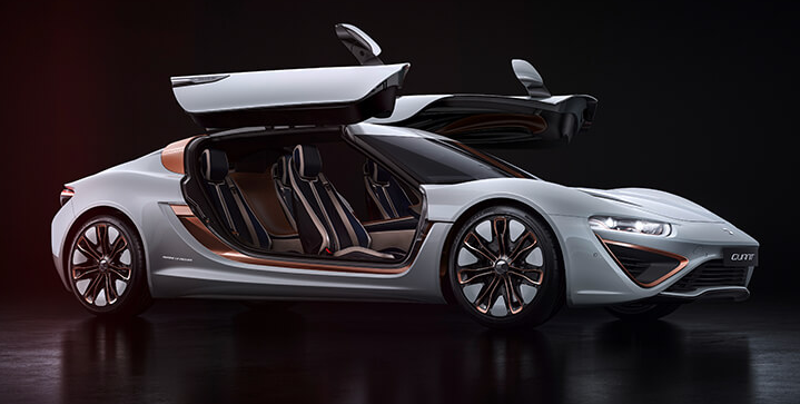 QUANT 48VOLT. Source: nanoFlowcell Holdings.
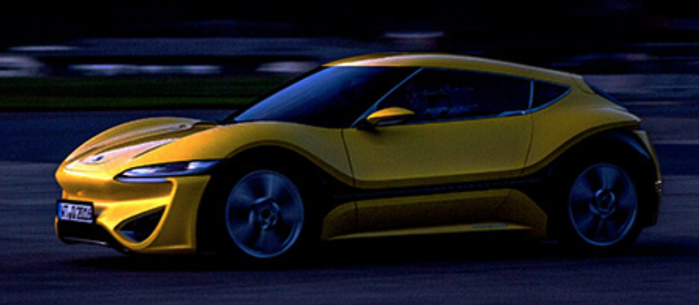 QUANTiNO. Source: nanoFlowcell Holdings.
In contrast to most other electric car manufacturers, nanoFlowcell Holdings has adopted a low voltage (48 volt) electric power system for which it claims the following significant benefits.
“The intrinsic safety of the nanoFlowcell® means its poles can be touched without danger to life and limb. In contrast to conventional lithium-ion battery systems, there is no risk of an electric shock to road users or first responders even in the event of a serious accident. Thermal runaway, as can occur with lithium-ion batteries and lead to the vehicle catching fire, is not structurally possible with a nanoFlowcell® 48VOLT drive. The bi-ION electrolyte liquid – the liquid “fuel” of the nanoFlowcell® – is neither flammable nor explosive. Furthermore, the electrolyte solution is in no way harmful to health or the environment. Even in the worst-case scenario, no danger could possibly arise from either the nanoFlowcell® 48VOLT low-voltage drive or the bi-ION electrolyte solution.”
In comparison, the more conventional lithium-ion battery systems in the Tesla, Nissan Leaf and BMW i3 electric cars typically operate in the 355 – 375 volt range and the Toyota Mirai hydrogen fuel cell electric power system operates at about 650 volts.
In the high-performance QUANT 48VOLT “supercar,” the low-voltage application of flow cell technology delivers extreme performance [560 kW (751 hp), 300 km/h (186 mph) top speed] and commendable range [ >1,000 kilometers (621 miles)]. The car’s four-wheel drive system is comprised of four 140 kW (188 hp), 45-phase, low-voltage motors and has been optimized to minimize the volume and weight of the power system relative to the previous high-voltage systems in the e-Sportlimousine and QUANT FE.
The smaller QUANTiNO is designed as a practical “every day driver.” You can read about a 2016 road test in Switzerland, which covered 1,167 km (725 miles) without refueling, at the following link:
http://emagazine.nanoflowcell.com/technology/1167-kilometre-test-drive-in-the-quantino/
A version of the QUANTiNO without supercapacitors currently is being tested. In this version, the energy for the electric motors comes directly from the flow cell battery, without any buffer storage in between. These tests are intended to refine the battery management system (BMS) and demonstrate the practicality of an even simpler, but lower performance, 48-volt power system.
Both the QUANT 48VOLT and QUANTiNO were represented at the 2017 Geneva Auto Show.
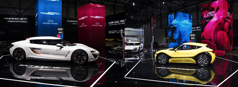 QUANT 48VOLT (left) and QUANTiNO (right). Source: nanoFlowcell Holdings.
You can read more about these cars at this auto show at the following link:
I think the automotive applications of flow cell battery technology look very promising, particularly with the long driving range possible with these batteries, the low environmental impact of the electrolytes, and the inherent safety of the low-voltage power system. I wouldn’t mind having a QUANT 48VOLT or QUANTiNO in my garage, as long as I could refuel at the end of a long trip.
Electrical utility-scale applications of flow cell batteries
In my 4 March 2016 post, “Dispatchable Power from Energy Storage Systems Help Maintain Grid Stability,” I noted that the reason we need dispatchable grid storage systems is because of the proliferation of grid-connected intermittent generators and the need for grid operators to manage grid stability regionally and across the nation. I also noted that battery storage is only one of several technologies available for grid-connected energy storage systems.
Flow cell battery technology has entered the market as a utility-scale energy storage / power system that offers some advantages over more conventional battery storage systems, such as the sodium-sulfur (NaS) battery system offered by Mitsubishi, the lithium-ion battery systems currently dominating this market, offered by GS Yuasa International Ltd. (system supplied by Mitsubishi), LG Chem, Tesla, and others, and the lithium iron phosphate (LiFePO4) battery system being tested in California’s GridSaverTM program. Flow cell battery advantages include:
- Flow cell batteries have no “memory effect” and are capable of more than 10,000 “charge cycles”. In comparison, the lifetime of lead-acid batteries is about 500 charge cycles and lithium-ion battery lifetime is about 1,000 charge cycles. While a 1,000 charge cycle lifetime may be adequate for automotive applications, this relatively short battery lifetime will require an inordinate number of battery replacements during the operating lifetime of a utility-scale, grid-connected energy storage system.
- The energy converter (the flow cell) and the energy storage medium (the electrolyte) are separate. The amount of energy stored is not dependent on the size of the battery cell, as it is for conventional battery systems. This allows better storage system scalability and optimization in terms of maximum power output (i.e., MW) vs. energy storage (i.e., MWh).
- No risk of thermal runaway, as may occur in lithium-ion battery systems
The firm UniEnergy Technologies (UET) offers two modular energy storage systems based on flow cell battery technology: ReFlex and the much larger Uni.System™, which can be applied in utility-scale dispatchable power systems. UET describes the Uni.System™ as follows:
“Each Uni.System™ delivers 600kW power and 2.2MWh maximum energy in a compact footprint of only five 20’ containers. Designed to be modular, multiple Uni.System can be deployed and operated with a density of more than 20 MW per acre, and 40 MW per acre if the containers are double-stacked.”
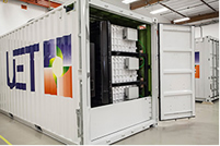 One Uni.System™ module. Source: UET
You can read more on the Uni.System™ at the following link:
http://www.uetechnologies.com/products/unisystem
The website Global Energy World reported that UET recently installed a 2 MW / 8 MWh vanadium flow battery system at a Snohomish Public Utility District (PUD) substation near Everett, Wash. This installation was one of five different energy storage projects awarded matching grants in 2014 through the state’s Clean Energy Fund. See the short article at the following link:
http://www.globalenergyworld.com/news/29516/Flow_Battery_Based_on_PNNL_Chemistry_Commissioned.htm
 Source: Snohomish PUD
Snohomish PUD concurrently is operating a modular, smaller (1 MW / 0.5 MWh) lithium ion battery energy storage installation. The PUD explains:
“The utility is managing its energy storage projects with an Energy Storage Optimizer (ESO), a software platform that runs in its control center and maximizes the economics of its projects by matching energy assets to the most valuable mix of options on a day-ahead, hour-ahead and real-time basis.”
You can read more about these Snohomish PUD energy storage systems at the following link:
http://www.snopud.com/PowerSupply/energystorage.ashx?p=2142
The design of both Snohomish PUD systems are based on the Modular Energy Storage Architecture (MESA), which is described as, “an open, non-proprietary set of specifications and standards developed by an industry consortium of electric utilities and technology suppliers. Through standardization, MESA accelerates interoperability, scalability, safety, quality, availability, and affordability in energy storage components and systems.” You’ll find more information on MESA standards here:
Application of the MESA standards should permit future system upgrades and module replacements as energy storage technologies mature.