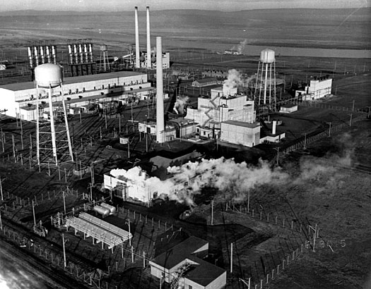
In the U.S., tritium for nuclear weapons was one of several products produced by the Atomic Energy Commission (AEC) and its successor, the Department of Energy (DOE), during the Cold War. The machines for tritium production were water-cooled, graphite-moderated production reactors in Hanford, Washington, and heavy water cooled and moderated production reactors at the Savannah River Plant (SRP, now Savannah River Site, SRS) in South Carolina. Lithium “targets,” containing enriched lithium-6 produced at the Y-12 Plant in Oak Ridge Tennessee, were irradiated in these reactors to produce tritium. Later, tritium was extracted from the targets, purified and packaged for use in nuclear weapons in separate facilities, initially at Hanford and Los Alamos and later at Savannah River.
Today, tritium for the U.S. nuclear weapons stockpile is produced in light water cooled and moderated commercial pressurized water reactors (PWRs) owned and operated by the Tennessee Valley Authority (TVA). Tritium is extracted from the targets, purified and packaged for use in nuclear weapons at the Savannah River Site (SRS).
The following three timelines provide details on tritium production activities in the Cold War nuclear weapons complex:
Under the Manhattan Project and through the Cold War, the U.S. developed and operated a dedicated nuclear weapons complex that performed all of the functions needed to transform raw materials into complete nuclear weapons. After the end of the Cold War (circa 1991), U.S. and Russian nuclear weapons stockpiles were greatly reduced. In the U.S., the nuclear weapons complex contracted and atrophied, with some functions being discontinued as the associated facilities were retired without replacement, while other functions continued at a reduced level, many in aging facilities.
In its current state, the U.S. nuclear weapons complex is struggling to deliver an adequate supply of tritium to meet the needs specified by the National Nuclear Security Administration (NNSA) for “stockpile stewardship and maintenance,” or in other words, for keeping the nuclear weapons in the current, smaller stockpile safe and operational. Key issues include:
There have been no dedicated tritium production reactors operating since 1988. Natural radioactive decay has been steadily reducing the existing inventory of tritium.
Commercial light water reactors (CLWRs) have been put into dual-use service since 2003 to produce tritium for NNSA while generating electric power that is sold commercially. The current tritium production rate needs to increase significantly to meet needs.
There has been a continuing decline in the national inventory of “unobligated” (i.e., free from peaceful use obligations) low-enriched uranium (LEU) and high-enriched uranium (HEU). This unobligated uranium can be used for military purposes, such as fueling the dual-use tritium production reactors.
There has been no “unobligated” U.S. uranium enrichment capability since 2013. The technology for a replacement enrichment facility has not yet been selected.
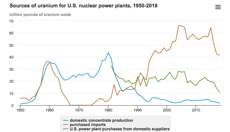
The U.S. domestic uranium production industry has declined to a small fraction of the capacity that existed from the mid-1950s to the mid-1980s. About 10% of uranium purchases in 2018 were from U.S. suppliers, and 90% came from other countries. NNSA’s new enrichment facility will need a domestic source of natural uranium.
There has been no operational lithium-6 production facility since the late 1980s.
There has been a continuing decline in the national inventory of enriched lithium-6, which is irradiated in “targets” to produce tritium.
Only one tritium extraction facility exists.
The U.S. nuclear weapons complex for tritium production is relatively fragile, with several milestone dates within the next decade that must be met in order to reach and sustain the desired tritium production capacity. There is little redundancy within this part of the nuclear weapons complex. Hence, tritium production is potentially vulnerable to the loss of a single key facility.
This complex story is organized in this post as follows.
Two key materials – Tritium and Lithium
Cold War tritium production
Hanford Project P-10 (later renamed P-10-X) for tritium production (1949 to 1954)
Hanford N-Reactor Coproduct Program for tritium production (1963 to 1967)
Savannah River Plant tritium production (1954 to 1988)
Synopsis of U.S. Cold War tritium production
The Interregnum of U.S Tritium Production (1988 to 2003)
New Production Reactor (NPR) Program
Accelerator Tritium Production (ATP)
Tritium recycling
The U.S. commercial light water reactor (CLWR) tritium production program (2003 to present)
Structure of the CLWR program
What is a TPBAR?
Operational use of TPBARs in TVA reactors
Where will the uranium fuel for the TVA reactors come from?
Tritium, or hydrogen-3, is naturally occurring in extremely small quantities (10-18 percent of naturally occurring hydrogen) or it can be artificially produced at great cost. The current tritium price is reported to be about $30,000 per gram, making it the most expensive substance by weight in the world today.
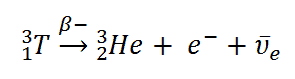
Tritium is a radioactive isotope of hydrogen with a half-life of 12.32 years. Tritium decays into helium-3 by means of negative beta decay, which also produces an electron (e–) and an electron antineutrino, as shown below.
Source: nuclear-power.net
Tritium is an important component of thermonuclear weapons. The tritium is stored in a small, sealed reservoir in each warhead.
With its relatively short half-life, the tritium content of the reservoir is depleted at a rate of 5.5% per year and must be replenished periodically. In 1999, DOE reported in DOE/EIS-0271 that none of the weapons in the U.S. nuclear arsenal would be capable of functioning as designed without tritium.
During the Cold War-era, the Atomic Energy Commission (AEC, and its successor in 1977, the Department of Energy, DOE) produced tritium for nuclear weapons in water-cooled, graphite-moderated production reactors in Hanford, Washington and in heavy water cooled and moderated production reactors at the Savannah River Plant (SRP, now Savannah River Site, SRS) in South Carolina. These reactors also produced plutonium, polonium and other nuclear materials. All of these production reactors were dedicated defense reactors except the dual-use Hanford-N reactor, which also could produce electricity for sale to the commercial power grid.
Tritium is produced by neutron absorption in a lithium-6 atom, which splits to form an atom of tritium (T) and an atom of helium-4. This process is shown below.
Natural lithium is composed of two stable isotopes; about 7.5% lithium-6 and 92.5% lithium-7. To improve tritium production, lithium-6 and lithium-7 are separated and the enriched lithium-6 is used to make “targets” that will be irradiated in nuclear reactors to produce tritium. The separated, enriched lithium-7 is a valuable material for other nuclear applications because of its very low neutron cross-section. Oak Ridge Materials Chemistry Division initiated work in 1949 to find a method to separate the lithium isotopes, with the primary goal of producing high purity lithium-7 for use in Aircraft Nuclear Propulsion (ANP) reactors.
Lithium-6 enrichment process development with a focus on tritium production began in 1950 at the Y-12 Plant in Oak Ridge, Tennessee. Three different enrichment processes would be developed with the goal of producing highly-enriched (30 to 95%) lithium-6: electric exchange (ELEX), organic exchange (OREX) and column exchange (COLEX). Pilot process lines (pilot plants) for all three processes were built and operated between 1951 and 1955.
Production-scale lithium-6 enrichment using the ELEX process was conducted at Y-12 from 1953 to 1956. The more efficient COLEX process operated at Y-12 from 1955 to 1963. By that time, a stockpile of enriched lithium-6 had been established at Oak Ridge, along with a stockpile of unprocessed natural lithium feed material.
The enriched lithium-6 material produced at Y-12 was shipped to manufacturing facilities at Hanford and Savannah River and incorporated into control rods and target elements that were inserted into a production reactor core and irradiated for a period of time.
After irradiation, these control rods and target elements were removed from the reactor and processed to recover the tritium that was produced. The recovered tritium was purified and then mixed with a specified amount of deuterium (hydrogen-2, 2H or D) before being loaded and sealed in reservoirs for nuclear weapons.
Tritium production at Hanford ended in 1967 and at Savannah River in 1988. The U.S. had no source of new tritium production for its nuclear weapons program between 1988 and 2003. During that period, tritium recycling from retired weapons was the primary source of tritium for the weapons remaining in the active stockpile. Finally, in 2003, the nation’s new replacement source of tritium for nuclear weapons started coming on line.
3. Cold War Tritium Production
3.1 Hanford Project P-10 (later renamed P-10-X) for tritium production (1949 to 1954)
The industrial process for producing plutonium for WW II nuclear weapons was conceived and built as part of the Manhattan Project. On 21 December 1942, the U.S. Army issued a contract to E. I. Du Pont de Nemours and Company (DuPont), stipulating that DuPont was in charge of designing, building and operating the future plutonium plant at a site still to be selected. The Hanford, Washington, site was selected in mid-January 1943.
Starting in 1949, the earliest work involving tritium production by irradiation of lithium targets in nuclear reactors was performed at Hanford under Project P-10 (later renamed P-10-X). By this time, DuPont had built and was operating four water-cooled, graphite-moderated production reactors at Hanford: B and D Reactors (1944), F Reactor (1945) and H Reactor (1949). Project P-10-X involved only the B and H Reactors, which were modified for tritium production.
Tritium was recovered from the targets in Building 108-B, which housed the first operational tritium extraction process line in the AEC’s nuclear weapons complex. The thermal extraction process employed started with melting the target material in a vacuum furnace and then collecting and purifying the tritium drawn off in the vacuum line. This tritium product was sent to Los Alamos for further processing and use.
Hanford site 100-B area. B Reactor is the tiered building near the center of the photo. The much smaller 108-B tritium extraction process line building is sitting alone on the right. Source: atomicarchive.com
Project P-10-X provided the initial U.S. tritium production capability from 1949 to 1954 and supplied the tritium for the first U.S. test of a thermonuclear device, Ivy Mike, in November 1952. Thereafter, most tritium production and all tritium extractions were accomplished at the Savannah River Plant.
DOE reported: “During its five years of operation, Project P-10-X extracted more than 11 million Curies (Ci) of tritium representing a delivered amount of product of about 1.2 kg.” For more details, see the report PNNL-15829, Appendix D: “Tritium Inventories Associated with Tritium Production,” which is available here:
3.2. Hanford N-Reactor Coproduct Program for tritium production (1963 to 1967)
This was a tritium production technology development program conducted in the mid-1960s. Its primary aim was not to produce tritium for the U.S. nuclear weapons program, but rather to develop technologies and materials that could be applied in tritium breeding blankets in fusion reactors. After an extensive review of candidate lithium-bearing target materials, the high melting point ceramic lithium aluminate (LiAlO2) was chosen.
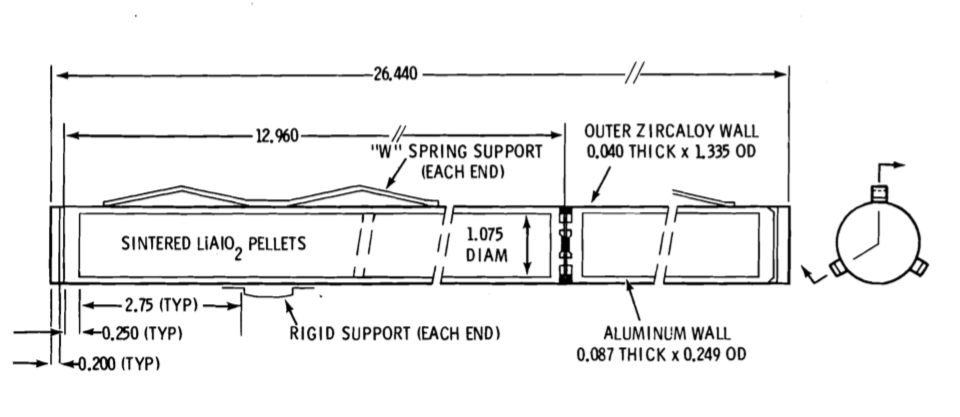
Several fuel-target element designs were tested in-reactor, culminating in October 1965 with the selection of the “Mark II” design for use in the full-reactor demonstration. Targets were double-clad cylindrical elements with a lithium aluminate core. The first cladding layer was 8001 aluminum; the second (outer) cladding layer was Zircaloy-2.
Hanford N Coproduct Target Element. Source: BNWL-2097
During the N Reactor coproduct demonstration, four distinct production tests were run, the first two with small numbers of fuel and target columns being irradiated, and the last two runs with over 1,500 fuel and target columns containing about 17 tons LiAlO2. The last production test, PT-NR-87, recorded the highest N Reactor power level by operating at 4,800 MWt for 31 hours.
The irradiated target elements were shipped to SRP for tritium extraction using a thermal extraction process defined jointly by Pacific Northwest Laboratory (PNL, now Pacific Northwest National Laboratory, PNNL) and Savannah River Laboratories (SRL). The existing tritium extraction vacuum furnaces at SRP were used.
This completed the Hanford N Reactor Coproduct Program.
More details are available in PNNL report BNWL-2097, “Tritium Production from Ceramic Targets: A Summary of the Hanford Coproduct Program,” which is available at the following link:
This program provided important experience related to lithium aluminate ceramic targets for tritium production.
3.3. Savannah River Plant tritium production (1954 to 1988)
The Savannah River Plant (SRP) was designed in 1950 primarily for a military mission to produce tritium, and secondarily to produce plutonium and other special nuclear materials, including Pu-238. DuPont built five dedicated production reactors at the SRP and became operational between 1953 and 1955: the R reactor (prototype) and the later P, L, K and C reactors.
In 1955, the original maximum power of C Reactor was 378 MWt. With ongoing reactor and system improvements, C Reactor was operating at 2,575 MWt in 1960, and eventually was rated for a peak power of 2,915 MWt in 1967. The other SRP production reactors received similar reactor and system improvements. The increased reactor power levels greatly increased the tritium production capacity at SRP. You’ll find SRP reactor operating power history charts in Chapter 2 of “The Savannah River Site Dose Reconstruction Project -Phase II,” report at the following link:
Enriched lithium-6 product was sent from the Oak Ridge Y-12 Plant to SRP Building 320-M, where it was alloyed with aluminum, cast into billets, extruded to the proper diameter, cut to the required length, canned in aluminum and assembled into control rods or “driver” fuel elements.From 1953 to 1955, tritium was produced only in control rods. Lithium-aluminum alloy target rods (“producer rods”) were installed in the septifoil (7-chambered) aluminum control rods in combination with cadmium neutron poison rods to get the desired reactivity control characteristics.
Cross-section of a septifoil control rod. Source: The Savannah River Site at Fifty (1950 – 2000), Chapter 13
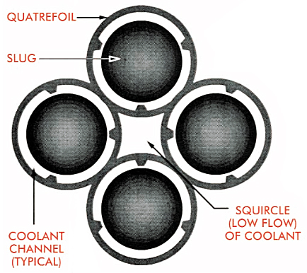
Starting in 1955, enriched uranium “driver” fuel cylinders and lithium target “slugs” were assembled in a quatrefoil (4-chambered) configuration, which provided much more target mass in the core for tritium production.
Cross-section of a quatrefoil driver fuel / target element. Source: The Savannah River Site at Fifty (1950 – 2000), Chapter 13
Enriched uranium drivers were extruded in Building 320-M until 1957, after which they were produced in the newly constructed Building 321-M. Production rate varied with the needs of the reactors, peaking in 1983, when the operations in Building 321-M went to 24 hours a day. Manufacturing ceased in 1989 after the last production reactors, K, L and P, were shut down.
K Reactor was operated briefly, and for the last time, in 1992 when it was connected to a new cooling tower that was built in anticipation of continued reactor operation. K Reactor was placed in cold-standby in 1993, but with no planned provision for restart as the nation’s last remaining source of new tritium production. In 1996, K Reactor was permanently shut down.
3.4. Synopsis of U.S. Cold War tritium production
The Federation of American Scientists (FAS) estimated that the total U.S. tritium production (uncorrected for radioactive decay) through 1984 was about 179 kg (about 396 pounds).
DOE reported a total of 10.6 kg (23.4 pounds) of tritium was produced at Hanford:
About 1.2 kg (2.7 pounds) was produced at the B and H Reactors during Project P-10-X.
The balance of Hanford production (9.4 kg, 20.7 pounds) is attributed to N Reactor operation during the Coproduct Program.
The majority of U.S. tritium production through 1984 occurred at the Savannah River Plant: about 168.4 kg (371.3 pounds).
4. The Interregnum of U.S Tritium Production (1988 – 2003)
DOE had shut down all of its Cold War-era production reactors. Tritium production at Hanford ended in 1967 and at Savannah River in 1988, leaving the U.S. temporarily with no source of new tritium for its nuclear weapons program. At the time, nobody thought that “temporary” meant 15 years (a period I call the “Interregnum”).
DOE’s search for new production capacity focused on four different reactor technologies and one particle accelerator technology. During the Interregnum, the primary source of tritium was from recycling tritium reservoirs from nuclear weapons that had been retired from the stockpile. This worked well at first, but tritium decays.
4.1 New Production Reactor (NPR) Program
From 1988 to 1992, DOE conducted the New Production Reactor (NPR) Program to evaluate four candidate technologies for a new generation of production reactors that were optimized for tritium production, but with the option to produce plutonium:
Heavy water cooled and moderated reactor (HWR)
High-temperature gas-cooled reactor (HTGR)
Light water cooled and moderated reactor (LWR)
Liquid metal reactor (LMR)
Three candidate NPR sites were considered:
Savannah River Site
Idaho National Engineering Laboratory (INEL, now INL)
Hanford Site
The NPR schedule goal was to have the new reactors start tritium production within 10 years after the start of conceptual design. Details on this program are available in DOE/NP-0007P, “New Production Reactors – Program Plan,” dated December 1990, which is available here: https://www.osti.gov/servlets/purl/6320732
The NPR program was cancelled in September 1992 (some say “deferred”) after DOE failed to select a preferred technology and failed to gain Congressional budgetary support for the program, at least in part due to the end of the Cold War.
DOE continued evaluating other options for tritium production, including commercial light water reactors (CLWRs) and accelerator tritium production (ATP).
4.2 Accelerator Tritium Production (ATP)
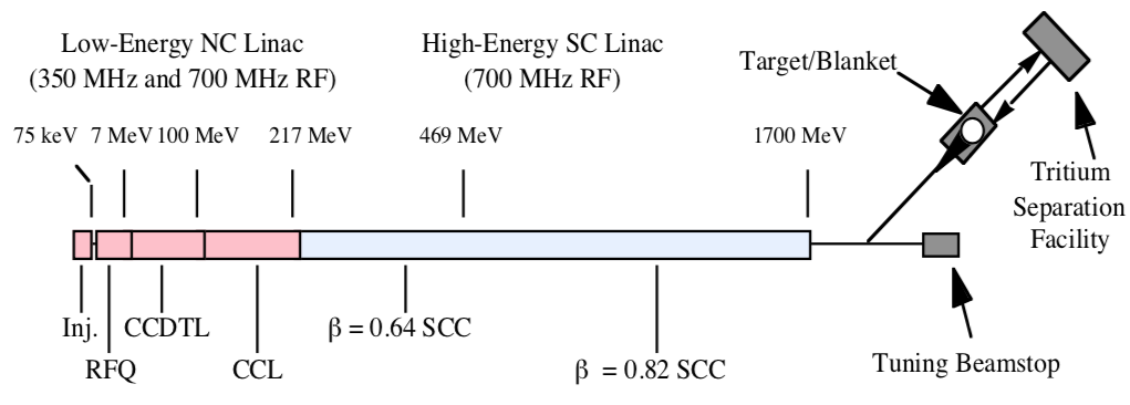
A candidate ATP design developed by Los Alamos National Laboratory (LANL) was based on a 1,700 MeV (million electron volt) linear accelerator that produced a 170 MW / 100 mA continuous proton beam. The ATP total electric power requirement was 486 MWe. The general arrangement of the ATP is shown in the following diagrams.
General arrangement of the ATP. Source: LANL
In this diagram, beam energy is indicated along the linear accelerator, increasing to the right and reaching a maximum of 1,700 MeV just before entering a magnetic switch that diverts the beam to the target/blanket or allows to beam to continue straight ahead to a tuning backstop.
Details of the Target / Blanket System. Source: LANL
The Target / Blanket System operates as follows:
The continuous proton beam is directed onto a tungsten target surrounded by a lead blanket, generating a huge flux of spallation neutrons.
Tubes filled with Helium-3 gas are located adjacent to the tungsten and within the lead blanket.
The spallation neutrons created by the energetic protons are moderated by the lead and cooling water and are absorbed by Helium-3 to create about 40 tritium atoms per incident proton.
The tritium is continuously removed from the Helium-3 gas in a nearby Tritium Separation Facility.
The unique feature of on-line, continuous tritium collection eliminates the time and processing required to extract tritium from the target elements used in production reactors.
ATP ultimately was rejected by DOE in December 1998 in favor of producing tritium in a commercial light water reactor (CLWR).
After the end of the Cold War, both the U.S. and Russia greatly reduced their respective stockpiles of nuclear weapons, as shown in the following chart.
Source: Wikipedia
The decommissioning of many nuclear weapons created an opportunity for the U.S. to temporarily maintain an adequate supply of tritium by recycling the tritium from the reservoirs no longer needed in warheads being retired from service. However, by 2020, after 32 years of exponential decay at a rate of 5.5% per year, the 1988 U.S. tritium inventory had decayed to only about 17% of the inventory in 1988, when the DOE stopped producing tritium. You can check my math using the following exponential decay formula:
y = a (1-b)x
where:
y = the fractional amount remaining after x periods
a = initial amount = 1
b = the decay rate per period (per year) = 0.055
x = number of periods (years) = 32
Recycling tritium from retired and aged reservoirs and precisely reloading reservoirs for installation in existing nuclear weapons are among the important functions performed today at DOE’s Savannah River Site (SRS). But, clearly, there is a point in time where simply recycling tritium reservoirs is no longer an adequate strategy for maintaining the current U.S. stockpile of nuclear weapons. A source of new tritium for military use was required.
5. The U.S. commercial light water reactor (CLWR) tritium production program (2003 to present)
In December 1998, Secretary of Energy Bill Richardson announced the decision to select commercial light water reactors (CLWRs) as the primary tritium supply technology, using government-owned Tennessee Valley Authority (TVA) reactors for irradiation services. A key commitment made by DOE was that the reactors would be required to use U.S.-origin low-enriched uranium (LEU) fuel. In their September 2018 report R45406, the Congressional Research Service noted: “Long-standing U.S. policy has sought to separate domestic nuclear power plants from the U.S. nuclear weapons program – this is not only an element of U.S. nuclear nonproliferation policy but also a result of foreign ‘peaceful-use obligations’ that constrain the use of foreign-origin nuclear materials.”
5.1 Structure of the CLWR program
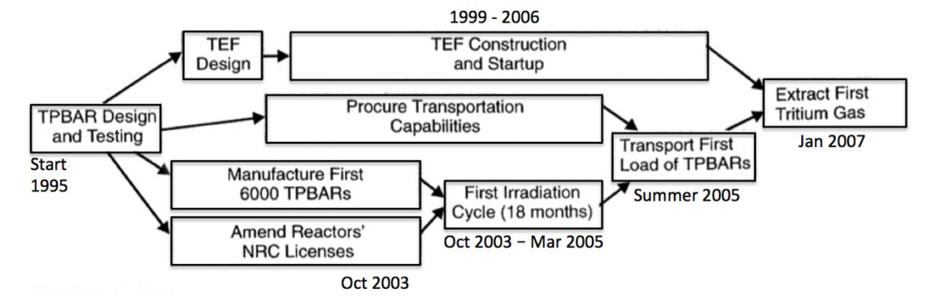
The current U.S. CLWR tritium production capability was deployed in about 12 years, between 1995 and 2007, as shown in the following high-level program plan.
CLWR tritium production program plan. Source: adapted from NNSA 2001
Since early 2007, NNSA has been getting its new tritium supply for nuclear stockpile maintenance from tritium-producing burnable absorber rods (TPBARs) that have been irradiated in the slightly-modified core of TVA’s Watts Bar Unit 1 (WBN 1) nuclear power plant, which is a Westinghouse commercial pressurized water reactor (PWR) licensed by the U.S. Nuclear Regulatory Commission (NRC).
TVA’s Watts Bar nuclear power plant. Source: Oak Ridge Today, 13 Feb 2019
The NRC’s June 2005 “Backgrounder” entitled, “Tritium Production,” provides a good synopsis of the development and nuclear licensing work that led to the approval of TVA nuclear power plants Watts Bar Unit 1 and Sequoyah Units 1 and 2 for use as irradiation sources for tritium production for NNSA. You find the NRC Backgrounder here:
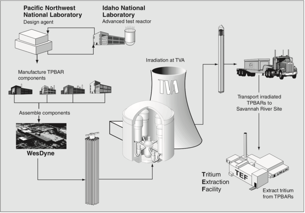
The CLWR tritium production cycle is shown in the following NNSA diagram. Not included in this diagram are the following:
Supply of U.S.-origin LEU for the fuel elements.
Production of fuel elements using this LEU
Management of irradiated fuel elements at the TVA reactor sites
The current U.S. tritium production cycle. Source: NNSA and Art Explosion via GAO-11-100
PNNL is the TPBAR design authority (agent) and is responsible for coordinating irradiation testing of TPBAR components in the Advanced Test Reactor (ATR) at the Idaho National Laboratory (INL). Production TPBAR components are manufactured by several contractors in accordance with specifications from PNNL, with WesDyne International responsible for assembling the complete TPBARs in Columbia, South Carolina. When needed, new TPBARs are shipped to TVA for installation in a designated reactor during a scheduled refueling outage and then irradiated for 18 months, until the next refueling outage. After being removed from the reactor, the irradiated TPBARs are allowed to cool at the TVA nuclear power plant for a period of time and then are shipped to the Savannah River Site.
SRS is the only facility in the nuclear security complex that has the capability to extract, recycle, purify, and reload tritium. Today, the Savannah River Tritium Enterprise (SRTE) is the collective term for the facilities, people, expertise, and activities at the SRS related to tritium production. SRTE is responsible for extracting new tritium from irradiated TPBARs at the Tritium Extraction Facility (TEF) that became operational in January 2007. They also are responsible for recycling tritium from reservoirs of existing warheads. The existing Tritium Loading Facility at SRS packages the tritium in sealed reservoirs for delivery to DoD. You’ll find the SRTE fact sheet at the following link:
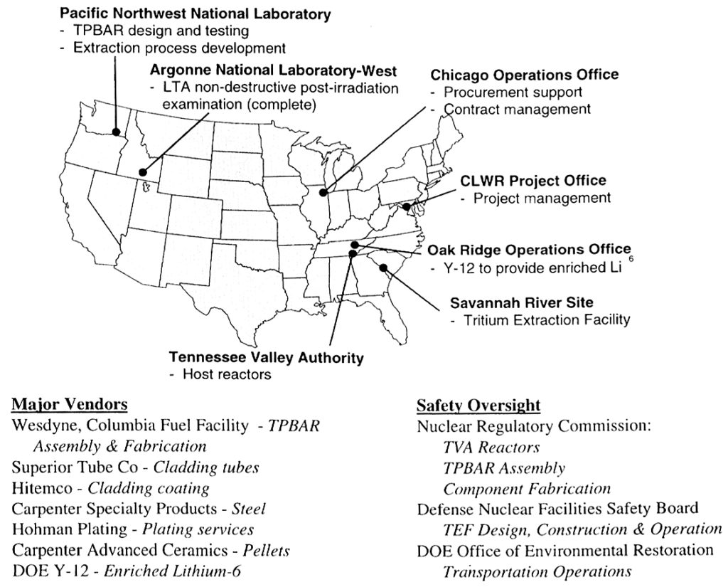
Program participants and their respective roles are identified in the following diagram.
The current U.S. tritium production program participants. Source: NNSA 2001
5.2 What is a TPBAR?
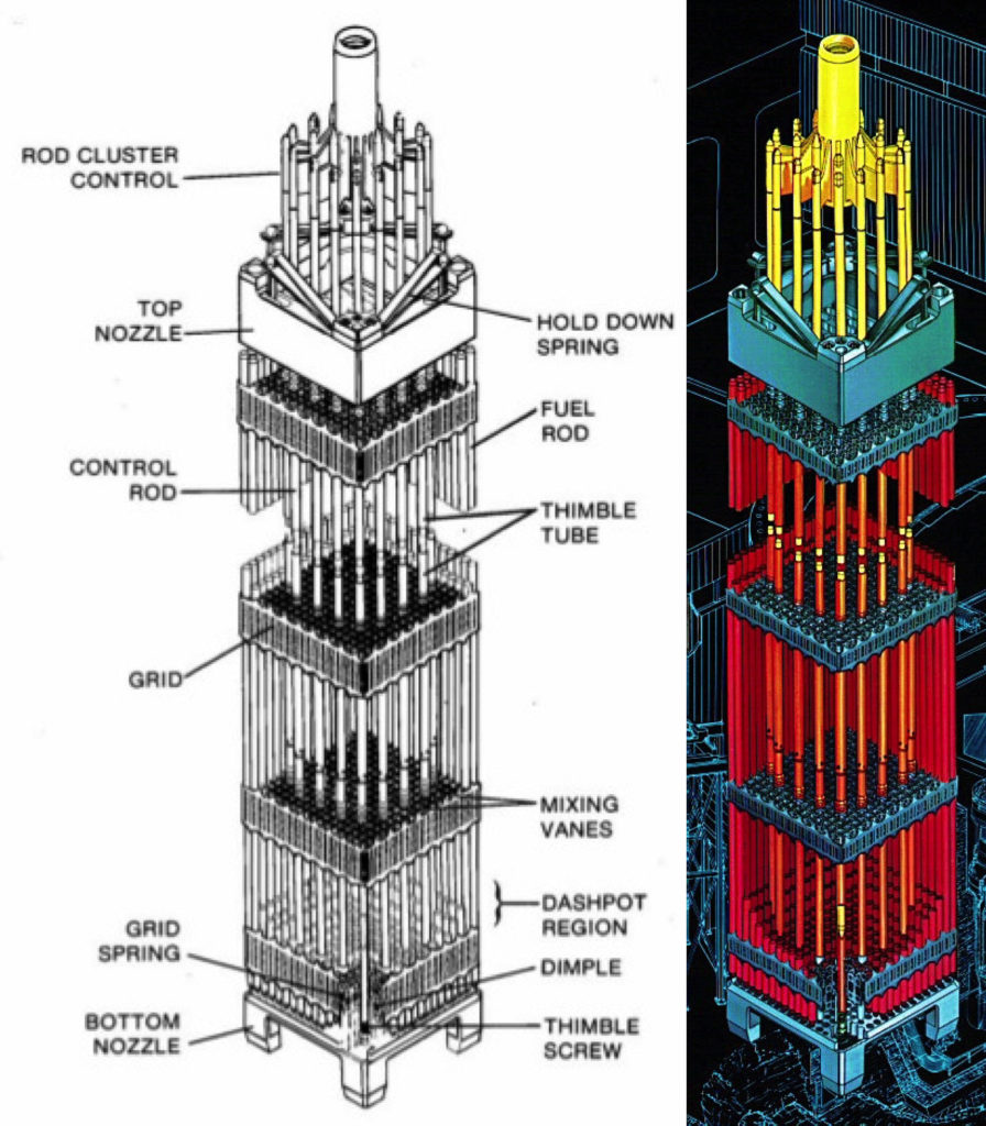
The reactor core in a Westinghouse commercial four-loop PWR like Watts Bar Unit 1 approximates a right circular cylinder with an active core measuring about 14 feet (4.3 meters) tall and 11.1 feet (3.4 meters) in diameter. The reactor core has 193 fuel elements, each of which is comprised of a 17 x 17 square array of 264 small-diameter, fixed fuel rods and 25 small-diameter empty thimbles, 24 of which serve as guide thimbles for control rods and one is an instrumentation thimble.
Rod cluster control assemblies (RCCAs) are used to control the reactor by moving arrays of small-diameter neutron-absorbing control rods into or out of selected fuel elements in the reactor core. Watts Bar has 57 RCCAs, each comprised of 24 Ag-In-Cd (silver-indium-cadmium) neutron-absorbing rods that fit into the control rod guide thimbles in selected fuel elements. Each RCCA is controlled by a separate control rod drive mechanism. The geometries of a Westinghouse 17 x 17 fuel element and the RCCA are shown in the following diagrams.
Cross-sectional view of a single Westinghouse 17 x 17 fuel element showing the lattice positions assigned to fuel rods (red) andthe thimbles available for instrumentation and control rods (blue).Source: Syeilendra Pramuditya Isometric view of a Westinghouse 17 x 17 fuel element showing the fixed fuel rods (red) and a rod cluster control assembly (yellow) that can be inserted or withdrawn for reactivity control. Sources: (L) Framatom ANP report BAW-10237, May 2001; (R) Westinghouse via NuclearTourist
To produce tritium in a Westinghouse PWR core, lithium-6 targets, in the form of lithium aluminate (LiAlO2) ceramic pellets, are inserted into the core and irradiated. This is accomplished with the tritium-producing burnable absorber rods (TPBARs), each of which is a small-diameter rod (a “rodlet”) that externally looks quite similar to a single control rod in an RCCA. During one typical 18-month refueling cycle (actually, up to 550 equivalent full power days), the tritium production per rod is expected to be in a range from 0.15 to 1.2 grams. The ceramic lithium aluminate target is similar to the targets developed in the mid-1960s and used during the Hanford N-Reactor Coproduct Program for tritium production.
A TPBAR “feed batch” assembly generally resembles the shape of an RCCA, but with 12 or 24 TPBAR rodlets in place of the control rods. The feed batch assembly is a hanging structure supported by the top nozzle adapter plate of the fuel assembly and the TPBAR rodlets are hanging in the guide thimble tubes of the fuel assembly. The feed batch assembly does not move after it has been installed in the reactor core.
Since lithium-6 is a strong neutron absorber, the TPBAR functions in the reactor core in a manner similar to fixed burnable absorber rods, which use boron-10 as their neutron absorber. The reactivity worth of the TPBARs is slightly greater than the burnable absorber rods.
In 2001, Framatome ANP issued Report BAW-10237, “Implementation and Utilization of Tritium Producing Burnable Absorber Rods (TPBARS) in Sequoyah Units 1 and 2.” This report provides a good description of the modified core and TPBARs as they would be applied for tritium production at the Sequoyah nuclear plant. Watts Bar should be similar. The report is here:
The feed batch assembly and TPBAR rodlet configurations are shown in the following diagram.
TPBAR feed batch assembly (left); details of an individual TPBAR and target pellet (right). Source: NNSA 2001
TPBARs were designed for a low rate of tritium permeation from the target pellets, through the cladding and into the primary coolant water. Tritium permeation performance was expected to be less than 1.0 Curie/one TPBAR rod/year. With an assumed maximum of 2,304 TPBARs in the reactor core, the NRC initially licensed Watts Bar Unit 1 for a maximum annual tritium permeation of 2,304 Curies / year.
5.3. Operational use of TPBARs in TVA reactors
NRC issued WBN 1 License Amendment 40 in September 2002, approving the irradiation of up to 2,304 TPBARs per operating cycle.
For the first irradiation cycle (Cycle 6) starting in the autumn of 2003, TVA received NRC approval to operate with only 240 TPBARs because of issues related to Reactor Coolant System (RCS) boron concentration. Actual TPBAR performance during Cycle 6 demonstrated a significantly higher rate of tritium permeation than expected; reported to be about 4.0 Curies/one TPBAR/cycle.
TVA’s short-term response was to limit the number of TPBARs per core load to 240 in Cycles 7 and 8 to ensure compliance with its NRC license limits on tritium release. In their 30 January 2015 letter to TVA, NRC stated, “….the primary constraint on the number of TPBARs in the core is the TPBAR tritium release per year of 2,304 Curies per year.” This guidance gave TVA some flexibility on the actual number of TPBARs that could be irradiated per cycle. This NRC letter is available here: https://www.nrc.gov/docs/ML1503/ML15030A508.pdf
PNNL’s examinations of TPBARs revealed no design or production flaws. Nonetheless, PNNL developed design modifications intended to improve tritium permeation performance. These changes were implemented by the manufacturing contractors, resulting in the Mark 9.2 TPBAR, which was first used in 2008 in WBN 1 Cycle 9. PNNL also is conducting an ongoing irradiation testing programs in the Advanced Test Reactor (ATR) at INL, with the goal of finding a technical solution for the high permeation rate. You’ll find details on this program in a 2013 PNNL presentation at the following link: https://www.energy.gov/sites/prod/files/2015/08/f26/Senor%20-%20TMIST-3%20Irradiation%20Experiment.pdf
In October 2010, the General Accounting Office (GAO) reported: “no discernable improvement in TPBAR performance was made and tritium is still permeating from the TPBARs at higher-than-expected rates.” This GAO report is available here: https://www.gao.gov/products/GAO-11-100
In response to the high tritium permeation rate, the irradiation management strategy was revised based on an assumed permeation rate of 5.0 Curies per TPBAR per year (five times the original expected rate). Even at this higher permeation rate, WBN 1 can meet the NRC requirements in 10 CFR Part 20 and 10 CFR Part 50 Appendix I related to controlling radioactive materials in gaseous and liquid effluents produced during normal conditions, including expected occurrences.
The many NRC license amendments associated with WBN 1 tritium production are summarized below:
In License Amendment 40 (Sep 2002), the NRC originally approved WBN 1 to operate with up to 2,304 TPBARs.
Cycle 6: TVA limited the maximum number of TPBARs to be irradiated to 240 based on issues related to Reactor Coolant System (RCS) boron concentration. Approved by NRC in WBN 1 License Amendment 48 (Oct 2003).
Cycles 7 & 8: WBN 1 continued operating with 240 TPBARs.
Cycle 9: First use of TPBARs Mark 9.2 supported TVAs request to increase the maximum number of TPBARs to 400. Approved by NRC in WBN 1 License Amendment 67 (Jan 2008)
Cycle 10: TVA reduced the number of TPBARs irradiated to 240 after discovering that the Mark 9.2 TPBAR design changes deployed in Cycle 9 did not significantly reduce tritium permeation.
Cycles 11 to 14: NRC License Amendment 77 9May 2009) allowed a maximum of 704 TPBARs at WBN 1. TVA chose to irradiate only 544 TPBARs in Cycles 11 and 12, increasing to 704 TPBARs for Cycles 13 & 14.
Cycles 15 & beyond: NRC License Amendment 107 (Aug 2016) allows a maximum of 1,792 TPBARs at WBN 1.
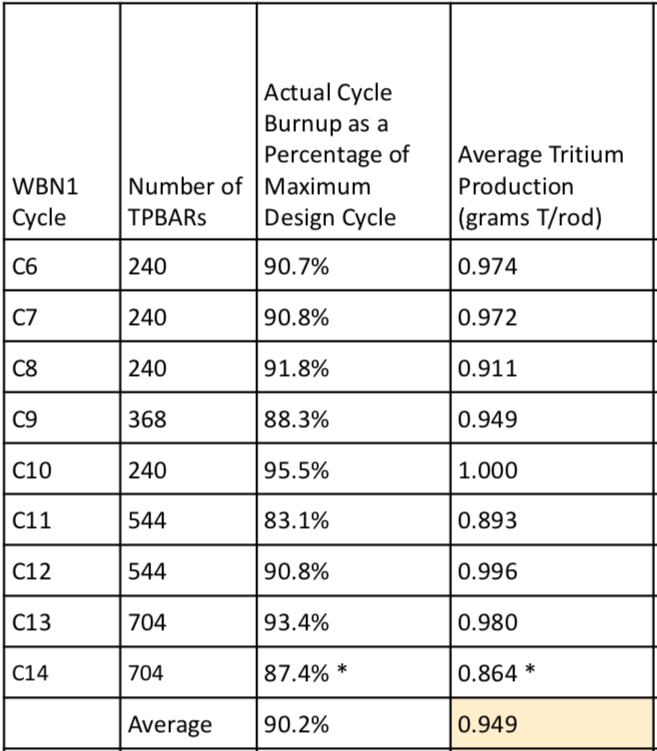
The actual number of TPBARs and the average tritium production per TPBAR during WBN 1 Cycles 6 to 14 are summarized in the 2017 PNNL presentation, “Tritium Production Assurance,” and are reproduced in the following table.
Tritium production, WBN 1 Cycles 6 to 14 (Cycle 14, completed in 2011, is an estimate). Source: PNNL, Tritium Production Assurance, 11 May 2017
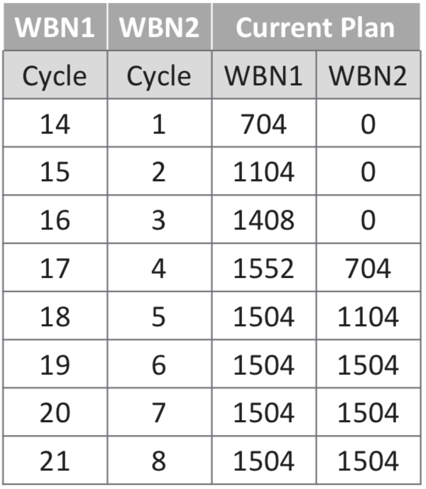
The current tritium production plan continues irradiation in WBN 1 and starts irradiation in Watts Bar Unit 2 (WBN 2) in Cycle 4, which will start after the spring 2022 refueling. Tritium is assumed to be delivered six months after the end of each cycle.
WBN 1 and WBN 2 TPBAR loading plans. Source: “Tritium Production Assurance”, report of the PNNL Tritium Focus Group, Richland, WA, May 11, 2017
As of early 2020, TVA and DOE are not delivering the quantity of tritium expected by NNSA. In July 2019, DOE and NNSA delivered their “Fiscal Year 2020 – Stockpile Stewardship and Management Plan” to Congress. In this plan, the top-level goal was to “recapitalize existing infrastructure to implement a plan to produce no less than 80 ppy (plutonium pits per year) by 2030.” To meet this goal, NNSA set a target for increasing tritium production to 2,800 grams per two 18-month reactor cycles of production at TVA by 2027. This means two TVA reactors will be producing tritium, and each will have a target of about 1,400 grams per cycle. This will be quite a challenge for TVA and DOE.
5.4 Where will the uranium fuel for the TVA reactors come from?
The tritium-producing TVA reactors are committed to using unobligated LEU fuel. That means that the uranium is not encumbered by international obligations that restrict its use for peaceful purposes only. Unobligated uranium has a very special pedigree. The uranium originated from U.S. mines, was processed in U.S. facilities, and was enriched in an unobligated U.S. enrichment facility.
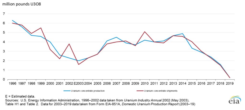
Today, that front-end of the U.S. nuclear fuel cycle has withered against international competition, as shown in the following chart from the Energy Information Administration (EIA).
Since the U.S. has not had an unobligated uranium enrichment facility since 2013, when the Paducah enrichment plant was closed by the Obama administration, there currently is no source of new unobligated LEU for the tritium-producing TVA reactors.
The impending shortage of unobligated enriched uranium eventually could affect tritium production, Navy nuclear reactor operation and other users. This matter has been addressed by the GAO in their 2018 report GAO-18-126, “NNSA Should Clarify Long-Term Uranium Enrichment Mission Needs and Improve Technology Cost Estimates,” which is available here:
The solution could be a mixture of measures, some of which are discussed briefly below.
Downblend unobligated HEU to buy time
Currently, the LEU for the TVA reactors is supplied from the U.S. inventory of unobligated LEU, which is supplemented by downblending unobligated HEU. In September 2018, NNSA awarded Nuclear Fuel Services (NFS) a $505 million contract to downblend 20.2 metric tons of HEU to produce LEU, which can serve as a short-term source of fuel for the tritium-producing TVA reactors. This contract runs from 2019 to 2025. Beyond 2025, additional HEU downblending may be needed to sustain tritium production until a longer-term solution is in place.
Build a new unobligated uranium enrichment facility and re-build the associated domestic uranium mining, milling and conversion infrastructure
NNSA is in the process of selecting the preferred technology for a new unobligated enrichment plant. There are two competing enrichment technologies: the Centrus AC-100 large advanced gas centrifuge and the Oak Ridge National Laboratory small advanced gas centrifuge, both of which are designed to enrich gaseous uranium hexafluoride (UF6).
NNSA failed to meet its goal of making the selection by the end of 2019. Regardless of the choice, it will take more than a decade to deploy such a facility. Perhaps a mid-2030’s date would be a possible target for initial operation of a new DOE uranium enrichment facility.
In the meantime, the atrophied / shutdown US uranium mining, milling and conversion industries need to be rebuilt to once again establish a reliable, domestic source of feed material for DOE’s uranium enrichment operations. This will be a daunting task given the current sad state of the US uranium production industry.
In May 2020, the US Energy Information Administration (EIA) released its 2019 Domestic Uranium Production Report. Mining uranium ore or in-situ leaching from underground uranium ore bodies, followed by the production of uranium (U3O8) concentrate (”yellowcake”), are the first steps at the front-end of the nuclear fuel cycle. The following EIA summary graphic shows the decline of US uranium production, which has been especially dramatic since 2013.
US uranium (U3O8) concentrate production and shipments, 1996–2019. Source: EIA
A key point reported by the EIA was that total US production of uranium concentrate from all domestic sources in 2019 was only 170,000 pounds (77,111 kg) of U3O8, 89% less than in 2018, from six facilities. In the graphic, you can see that US annual production in 1996 was about 35 times greater, approximately 6,000,000 pounds (2,721,554 kg). This EIA report is available at the following link: https://www.eia.gov/uranium/production/annual/
Conversion of U3O8 to UF6 is the next step in the front-end of the nuclear fuel cycle. Honeywell’s Metropolis Works was built in 1958 to produce UF6 for US government programs, including the nuclear weapons complex. Therefore, the Metropolis Works should be an unobligated conversion plant and, as such, is an important facility in the nuclear fuel cycle for the US tritium production reactors operated by TVA. In 2020, the Metropolis Works is the only US facility that can receives uranium ore concentrate and convert it to UF6.
In 1968, Metropolis Works began selling UF6 on the commercial nuclear market. However, since 2017, operations at the Metropolis Works have been curtailed due to weak market conditions for its conversion services and Honeywell has maintained the facility in a “ready-idle” status. In March 2020, the NRC granted the Metropolis Works a 40-year license renewal, permitting operations until March 24, 2060. When demand resumes, the Metropolis Works should be ready to resume operation.
Recognizing the US national interest in having a viable industrial base for the front-end of the nuclear fuel cycle, President Trump established a Nuclear Fuel Working Group in July 2019. On 13 April, 2020, the DOE released the “Strategy to Restore American Nuclear Energy Leadership,” which, among other things, includes recommendations to strengthen the US uranium mining and conversion industries and restore the viability of the entire front-end of the nuclear fuel cycle. You’ll find this DOE announcement and a link to the full report to the President here: https://www.energy.gov/articles/secretary-brouillette-announces-nuclear-fuel-working-groups-strategy-restore-american
Reprocess enriched DOE and naval fuel spent fuel
A large inventory of aluminum clad irradiated fuel exists at SRS, with a smaller quantity at INL. The only operating chemical separations (reprocessing) facility in the U.S. is the H-Canyon facility at SRS, which can only process aluminum clad fuel. However, the cost to operate H-Canyon to process the aluminum-clad fuel would be high.
There is a large inventory of irradiated, zirconium-clad naval fuel at INL. This fuel started life with a uranium enrichment level of 93% or higher. In 2017, INL completed a study examining the feasibility of processing zirconium-clad spent fuel through a new process called ZIRCEX. This process could enable reprocessing the spent naval fuel stored at INL as well as other types of zirconium-clad fuel.
In 2018, the U.S. Senate approved $15 million in funding for a pilot program at the INL to “recycle” irradiated (used) naval nuclear fuel and produce high-assay, low-enriched uranium (HALEU) fuel with an enrichment between 5% to 20% for use in “advanced reactors.” It seems that a logical extension would be to also produce LEU fuel to a specification that could be used in the TVA reactors.
In 2018, Idaho Senator Mike Crapo made the following report to the Senate: “HEU repurposing, from materials like spent naval fuel, can be done using hybrid processes that use advanced dry head-end technologies followed by material recovery, which creates the fuel for our new advanced reactors. Repurposing this spent fuel has the potential of reducing waste that would otherwise be disposed of at taxpayer expense, and approximately 1 metric ton of HEU can create 4 useable tons (of HALEU) for our new reactors.”
Perhaps there is a future for closing the back-end of the naval fuel cycle and recovering some of the investment that went into producing the very highly enriched uranium used in naval reactors. Because of the high burnup in long-life naval reactors, the resulting HALEU or LEU will have different uranium isotopic proportions than LEU produced in the front-end of the fuel cycle. This may introduce issues that would have to be reviewed and approved by the NRC before such LEU fuel could be used in the TVA reactors.
Other options
More information on options for obtaining enriched uranium without acquiring a new uranium enrichment facility is provided in Appendix II of GAO-18-126.
5.5 Where will the enriched lithium-6 target material come from?
A reliable source of lithium-6 target material is needed to produce the TPBARs for TVA’s tritium-producing reactors.
The U.S. has not had an operational lithium-6 production facility since 1963 when the last COLEX (column exchange) enrichment line was shutdown. COLEX was one of three lithium enrichment technologies employed at the Y-12 Plant in Oak Ridge, TN between 1950 and 1963. The others technologies were ELEX (electrical exchange) and OREX (organic exchange). All of these processes used large quantities of mercury. At the time lithium-6 enrichment operations ceased at Y-12, a stockpile of enriched lithium-6 and lithium-7 had been established along with a stockpile of unprocessed natural lithium feed material.
There has been a continuing decline in the national inventory of enriched lithium-6. To extend the existing supply, NNSA has instituted a program to recover and recycle lithium components from nuclear weapons that are being retired from the stockpile.
In May 2017, Y-12 lithium activities were adversely affected by the poor physical condition (and partial roof collapse) of the WW II-vintage Building 9204-2 (Beta 2).
Shortly thereafter, NNSA announced the approval of plans for a new Lithium Production Facility at Y-12 to replace Building 9204-2. The NNSA’s Fiscal Year 2020 – Stockpile Stewardship and Management Plan set an operational date of 2030 for the new facility.
5.6 Where is the tritium recovered?
Tritium is extracted from the irradiated TPBARs, purified and loaded into reservoirs at the Savannah River Site (SRS). These functions are performed by “Savannah River Tritium Enterprise” (SRTE), which is the collective term for the tritium facilities, people, expertise, and activities at the SRS.
The first load of irradiated TPBARs were consolidated at Watts Bar and delivered to SRS in August 2005 for storage pending completion of the new Tritium Extraction Facility (TEF). The TEF became fully operational and started extracting tritium from TPBARs in January 2007. The tritium extracted at TEF is transferred to the H Area New Manufacturing (HANM) Facility for purification. In February 2007, the first newly-produced tritium was delivered to the SRS Tritium Loading Facility for loading into reservoirs for nuclear weapons.
From 2007 until 2017, the TEF conducted only a single extraction each year because of the limited quantities of TPBARs being irradiated in the TVA reactors. During this period, the TEF sat idle for nine months each year between extraction cycles.
In 2017, for the first time, the TEF performed three extractions in a single year using the original vacuum furnace. Each extraction typically involved 300 TPBARs.
In November 2019, SRTE’s capacity for processing TPBARs and recovering tritium was increased by the addition of a second vacuum furnace.
6. Conclusions
In their “Fiscal Year 2020 – Stockpile Stewardship and Management Plan,” the NNSA’s top-level goal is to “recapitalize existing infrastructure to implement a plan to produce no less than 80 ppy (plutonium pits per year) by 2030.” This goal will drive tritium production demand, which in turn will drive demands for unobligated LEU to fuel TVA’s tritium-producing reactors and enriched lithium-6 for TPBARs.
The U.S. nuclear fuel cycle for the production of tritium currently is incomplete. It is able to produce tritium by using temporary measures that are not sustainable:
Downblending HEU to produce LEU
Recycling tritium as the primary means for meeting current demand
Recycling lithium components
The next 15 years will be quite a challenge for the NNSA, DOE and TVA as they work to reestablish a complete, modern nuclear fuel cycle for tritium production. There are several milestones on the critical path that would adversely impact tritium production if they are not met on schedule:
Higher tritium production goals for the TVA reactors: deliver 2,800 grams of tritium per two 18-month reactor cycles of production in TVA reactors by 2027
New Lithium Facility at Y-12 operational by 2030
New uranium enrichment facility operational, perhaps by the mid-2030s
There is a general lack of redundancy in the existing and planned future nuclear fuel cycle for tritium production. This makes tritium production vulnerable to a major outage at a single non-redundant facility.
“National Nuclear Security Administration Needs to Ensure Continued Availability of Tritium for the Weapons Stockpile,” Report GAO-11-100, General Accounting Office, October 2010: https://www.gao.gov/assets/320/311092.pdf
Sean Johnson, “Making the invisible engineer visible: DuPont and the recognition of nuclear expertise,” Technology and Culture, Volume 52, Number 3, July 2011, pp. 548-573: https://muse.jhu.edu/article/447781/pdf
For more information on Cold War-era Hanford tritium production:
Johnson AB, Jr., TJ Kabele, and WE Gurwell, “Tritium Production from Ceramic Targets: A Summary of the Hanford Coproduct Program,” BNWL-2097, Pacific Northwest National Laboratory, 1976: https://www.osti.gov/servlets/purl/7125831
Johnson AB, Jr., TJ Kabele, and WE Gurwell, “Tritium Production from Ceramic Targets: A Summary of the Hanford Coproduct Program,” BNWL-2097, Pacific Northwest National Laboratory, 1976: https://www.osti.gov/servlets/purl/7125831
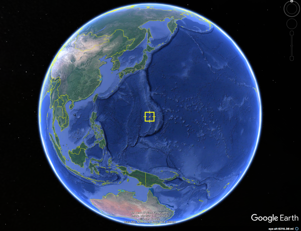
The Challenger Deep, in the Mariana Trench in the middle of western Pacific Ocean, is the deepest known area in the world’s oceans. Its location, as shown in the following map, is 322 km (200 miles) southwest of Guam and 200 km (124 miles) off the coast of the Mariana Islands.
Location of the Mariana Trench. Source: Google Earth
Since the first visit to the bottom of the Challenger Deep 60 years ago, on 23 January 1960, there have been only five other visits to that very remote and inhospitable location. In this post, we’ll take a look at the deep-submergence vehicles (DSVs) and the people who made these visits.
The following topographical map, created in 2019 by the Five Deeps Expedition, shows that the Challenger Deep is comprised of three deeper “pools.” The dive locations of the manned expeditions into the Challenger Deep are shown on this map.
1960: Navy Lieutenant Don Walsh and Swiss engineer Jacques Piccard, in the bathyscaphe Trieste, made the first manned descent into the Challenger Deep and reached the bottom at 10,916 meters (35,814 ft) in the “Western Pool.”
2012: Canadian filmmaker and National Geographic Explorer-in-Residence James Cameron, in the DSV Deepsea Challenger, reached the bottom at 10,908 meters (35,787 ft) the “Eastern Pool.”
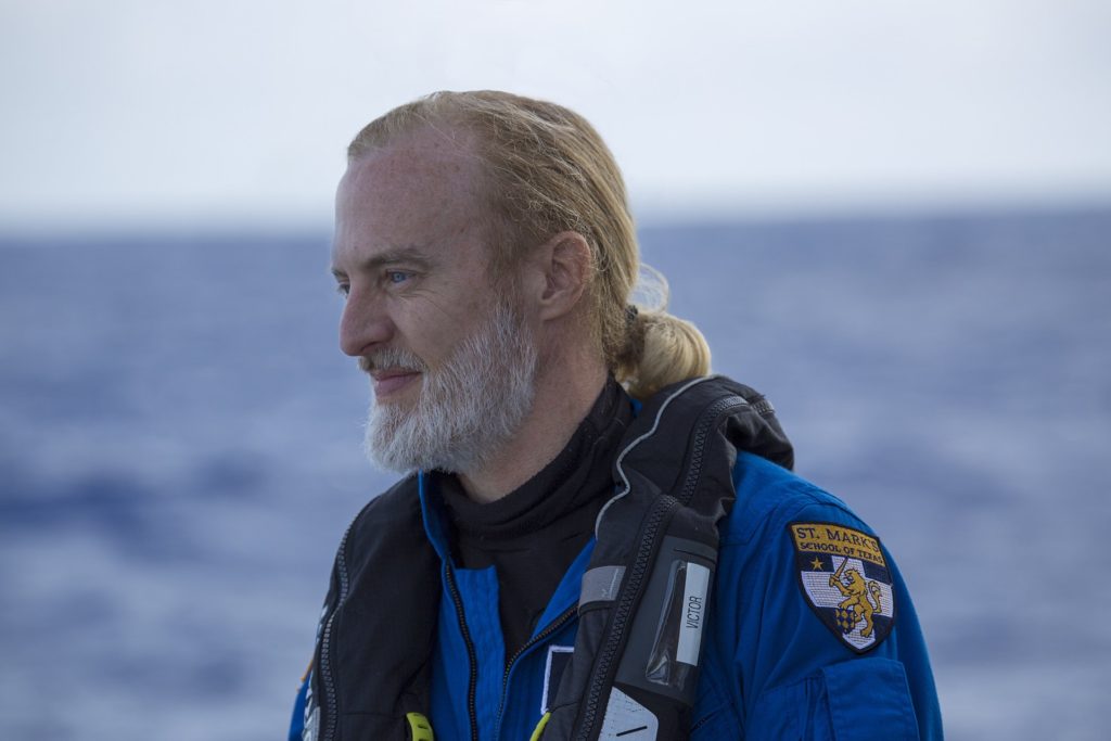
2019: Businessman, explorer and retired naval officer Victor Vescovo, in the DSV Limiting Factor, made two dives in the “Eastern Pool” and reached a maximum depth of 10,925 meters (35,843 feet).
2019: Triton Submarine president, Patrick Lahey, in the DSV Limiting Factor, made two dives to the bottom, one in the Eastern Pool and one in the Central Pool.
Topography of the Challenger Deep and locations of the deep dive sites. Source: Five Deeps Expedition
What is there to see on the way down to the bottom?
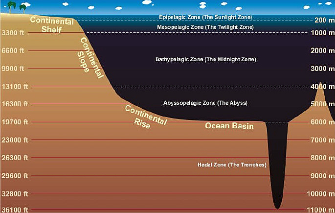
The oceans can be divided into vertical zones based on water depth. This basic concept is shown in the following diagram.
The five vertical zones in the above diagram have the following general characteristics:
The Sunlight Zone: This is the shallow (upper 150 meters), sunlit upper layer of the ocean, extending above the continental shelf. Phytoplankton can photosynthesize in this zone.
The Twilight Zone: This is the medium-depth ocean where sunlight is still able to penetrate to a modest depth (a few hundred meters). There is enough light to see, but not enough for photosynthesis. This zone is bounded by the edges of the continental shelf and islands in the deep ocean.
The Midnight Zone: This is the deep ocean, which is bounded by the continental slope and the seamounts and islands rising above the ocean floor. No sunlight is able to reach this deep. There is no photosynthesis in this zone.
The Abyssal Zone: This zone includes the deep ocean plains and the deep cusp of the continental rise. The temperature here is near freezing and very few animals can survive the extreme pressure.
The Hadal Zone: This is the ocean realm in the deep ocean trenches. More people have been to the Moon than to the Hadal Zone.
The Challenger Deep is the deepest known Hadal Zone on our planet. On the way down through 11 kilometers (6.8 miles) of ocean, the few explorers who have reached the bottom have seen aquatic life throughout the water column and on the sea floor. You can take a look the varied and strange sea life by scrolling through the well done graphic, “The Deep Sea,” by Neal Agarwal, which is at the following link.
Now, let’s take a look at the few manned missions that have reached the bottom of the Challenger Deep.
1960: Jacques Piccard and Don Walsh in the bathyscaphe Trieste
Trieste was designed by Swiss scientist Auguste Piccard and was built in Italy. This deep-diving research bathyscaphe enabled the operators to make a free dive into the ocean, without support by cables from the surface. Trieste was launched in August 1953, operated initially by the French Navy and acquired by the U.S. Navy in 1958.
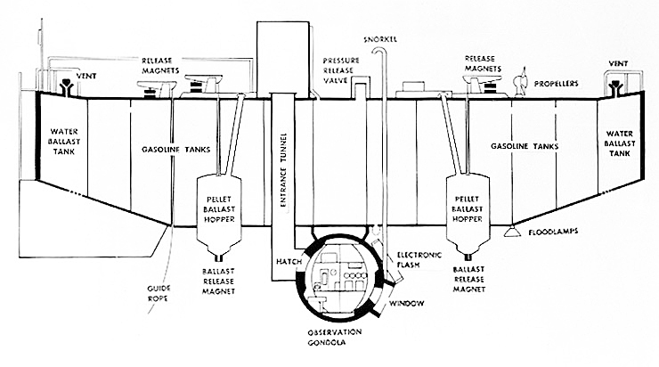
The design of the 15 meter (50 ft) bathyscaphe Trieste is analogous to a zeppelin that has been redesigned to operate underwater. On Trieste, the “gondola” is a 14-ton spherical steel pressure vessel for two crew members. The weight of this “gondola” is carried under a large, lightweight, cylindrical float chamber filled with gasoline for buoyancy (gasoline is less dense than water). There is no differential pressure between the float chamber and the open ocean.
General arrangement of the bathyscaphe Trieste. Source: National Geographic
The Trieste is positively buoyant when loaded with ballast and floating on the surface before a mission. To submerge, Trieste would take on seawater and fill its fore and aft water ballast tanks. If needed to achieve the desired negative buoyancy, Trieste also could release some gasoline from the main float chamber. To achieve positive buoyancy at the end of a mission and ascend back to the surface, the pellets in the two ballast hoppers would be released, and Trieste would slowly rise to the surface.
The propulsion system consists of five special General Electric 3-hp dc motors. These motors are designed to operate in inert fluid (silicone oil) and are subjected to full ambient pressure during diving operations. These modest propulsors gave Trieste only limited mobility.
After acquisition by the Navy, Trieste was transported to San Diego, CA, for extensive modifications by the Naval Electronics Laboratory.
After a series of local dives in Southern California waters, Trieste departed San Diego on 5 October 1959 aboard a freighter and was transported to Guam to conduct deep dives in the Pacific Ocean under Project Nekton. After arriving in Guam, record-setting dives to 18,000 and 24,000 feet were conducted in nearby waters by Navy Lieutenant Don Walsh and Swiss engineer Jacques Piccard (son of Auguste Piccard). Then Trieste was towed to the Mariana Trench dive site, where Walsh and Piccard began their mission into the Challenger Deep on 23 January 1960.
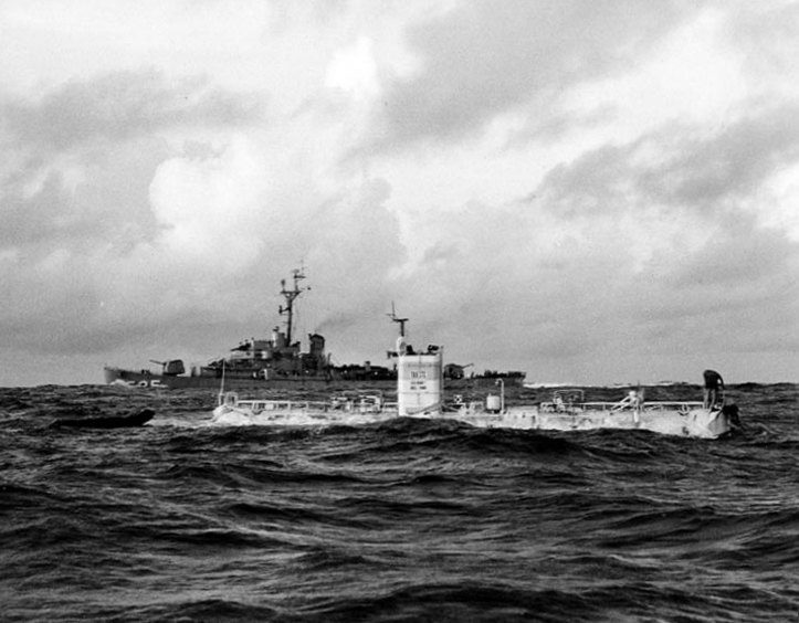
Trieste just before the record dive on 23 January 1960. The destroyer escort USS Lewis is in the background. Source: U.S. Navy photo.
Don Walsh (L) and Jacques Piccard (R) aboard Trieste. Source: U.S. Navy photo.
The mission took 8 hours and 22 minutes on the following timeline:
Descent to the ocean floor took 4 hours 47 minutes. They reached the bottom at a depth of 10,916 meters (35,814 ft).
Time on the bottom was 20 minutes.
Ascent took 3 hours and 15 minutes.
For much of the mission, cabin temperature was about 7° C (45° F). While on the bottom, Walsh and Piccard observed sea life, although the species observed are uncertain. They described the sea bottom as a “diatomaceous ooze.”
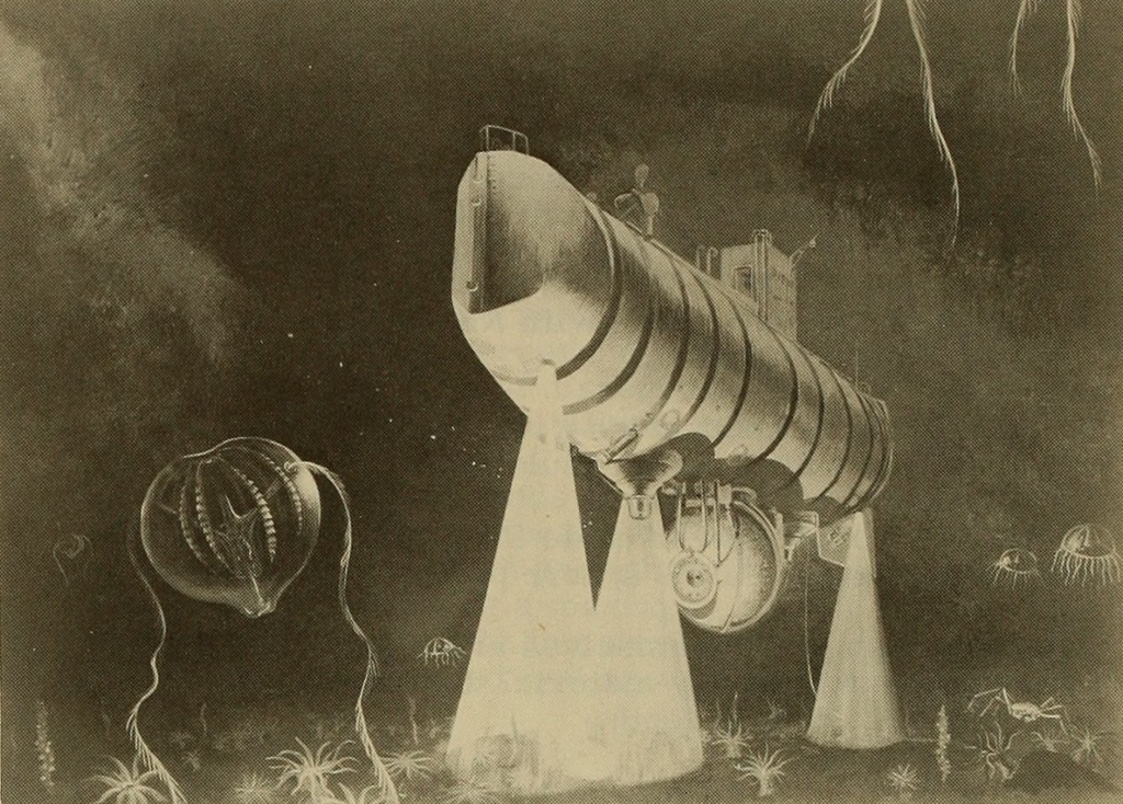
Artist’s concept drawing of Trieste on the bottom. Source: Internet Archive, page 21 of the book “The bathyscaph Trieste : technological and operational aspects, 1958-1961,” (1962) by Don Walsh
For a comprehensive review of this historic dive into the Challenger Deep, I recommend that you watch the following video, “Rolex presents: The Trieste’s Deepest Dive,” (22:38).
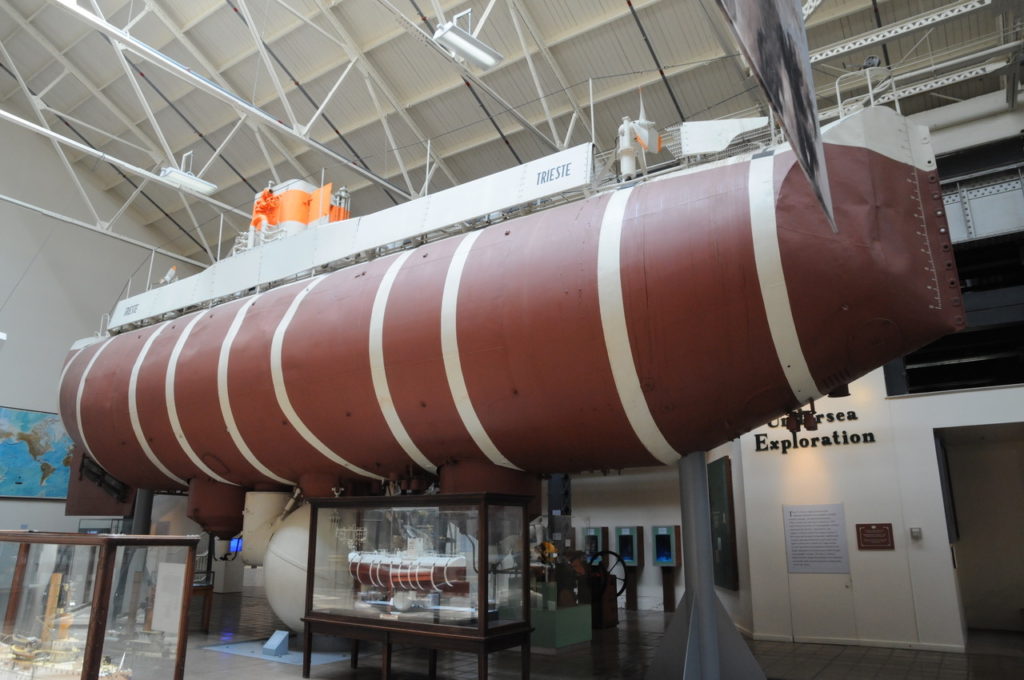
After successfully completing Project Nekton, Trieste underwent further modifications and was transferred to the East Coast in 1963 to assist in the search for the USS Thresher (SSN-593), which sank off the coast of New England. Trieste found the wreck of the nuclear submarine at a depth of 2,600 m (8,400 ft). Trieste was decommissioned in 1966 and went on display in 1980 at the National Museum of the U.S. Navy in Washington, D.C. Following are photos I took during my visit to that museum.
Trieste bow quarter view, at the National Museum of the U.S. Navy. P. Lobner photo
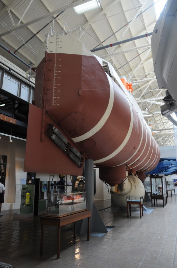
Trieste stern quarter view. P. Lobner photo
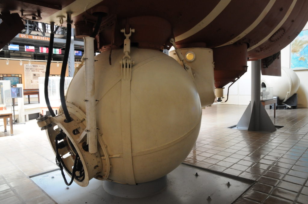
Trieste crew pressure vessel. P. Lobner photo.
2012: James Cameron in the Deepsea Challenger
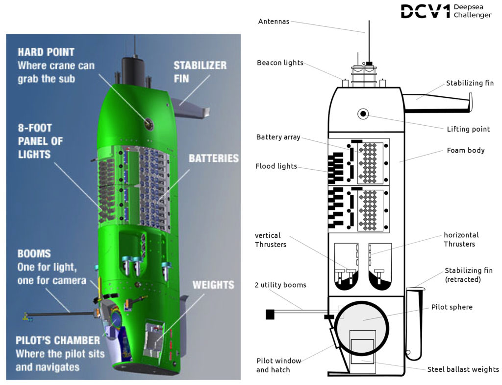
Almost a decade ago, filmmaker and National Geographic Explorer-in-Residence James Cameron led a team that designed and built the one-man, 11.8-ton DSV named Deepsea Challenger (DCV 1) for a mission to dive into the Challenger Deep and reach the deepest point in the ocean. The general arrangement of this novel submersible is shown in the following diagram.
General arrangement of the Deepsea Challenger. Sources: https://www.core77.com (left), Wikipedia (right)
In the water, the submersible floats vertically with the steel pilot’s chamber at the bottom of the vessel. When brought aboard its support vessel, the submersible sits horizontally in a cradle.
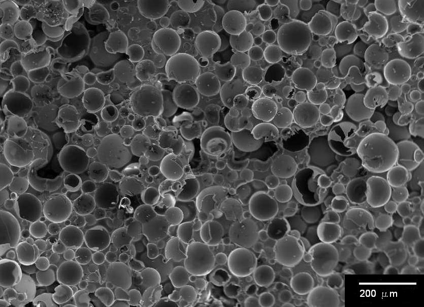
About 70% of the Deepsea Challenger’s volume is comprised of a specialized structural syntactic foam called Isofloat, which is composed of very small hollow glass spheres suspended in an epoxy resin.
Syntactic foam, shown by scanning electron microscopy, consisting of glass microspheres within a matrix of epoxy resin. Source: Nikgupt via Wikipedia
The strength of this structural foam enabled the designers to incorporate 12 thrusters as part of the infrastructure mounted within the foam, but without the need for a steel skeleton to handle the loads from the various mechanisms. The lithium batteries are housed within the syntactic foam structure. The foam also provides buoyancy, like the gasoline-filled float chamber on the bathyscaphe Trieste.
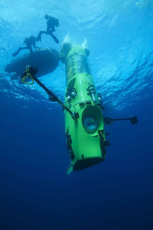
The Deepsea Challenger is equipped with a sediment sampler, a robotic claw, temperature, salinity, and pressure gauges, multiple 3-D cameras and an 8-foot (2.5-meter) tower of LED lights. An underwater acoustic communication system provides the communications link with the support vessel during the dive. Mission endurance is 56 hours.
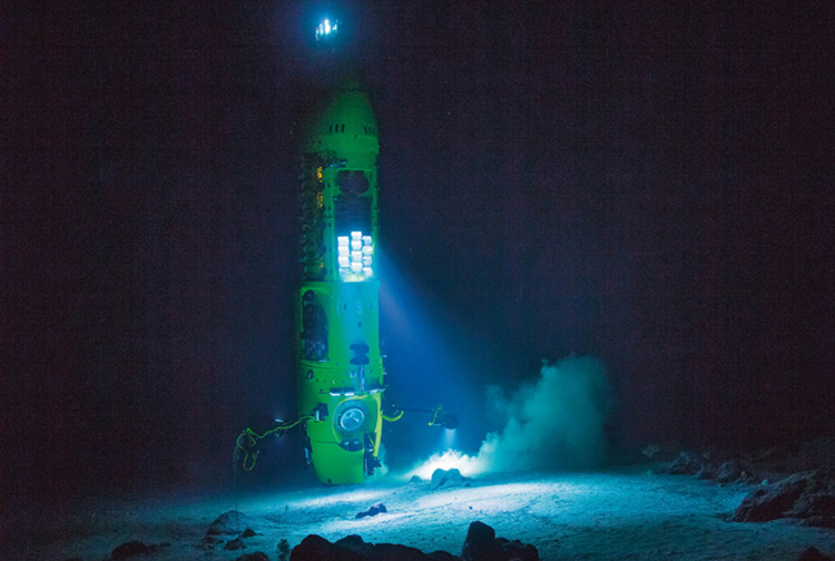
Deepsea Challenger floating vertically in the water with booms extended.Source: National Geographic
On March 26, 2012, more than 52 years after the Trieste’s dive into the Challenger Deep, Cameron plunged 10,908 meters (35,787 feet, 11 kilometers, 6.8 miles) below the ocean surface and became the first solo diver to reach such depths. After a two hour and 36 minute descent, he traveled along the bottom for about three hours and reported it being a flat plain with a soft, gelatinous sea floor. The thrusters enabled precise station keeping and a maximum speed of 3 knots.
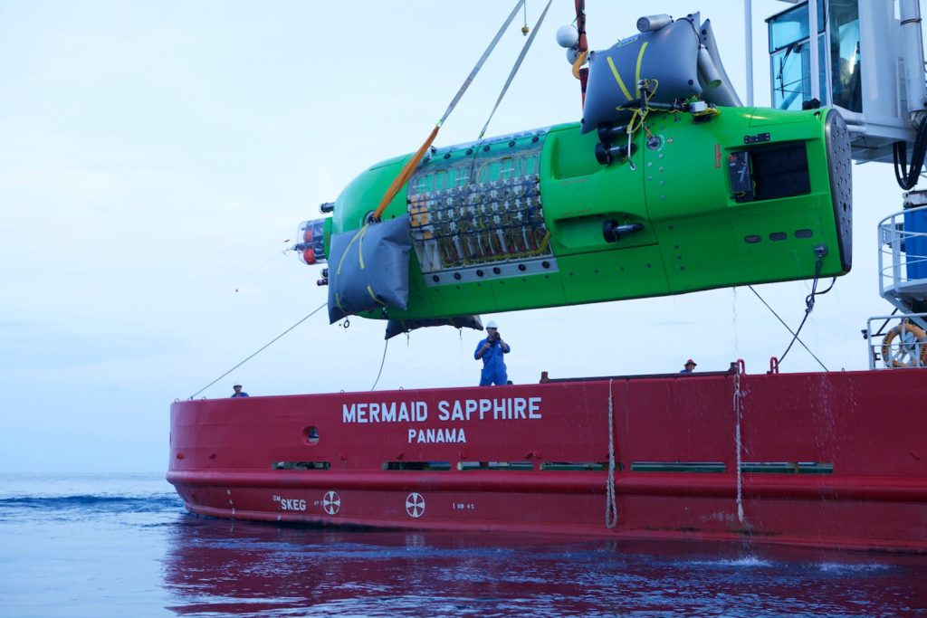
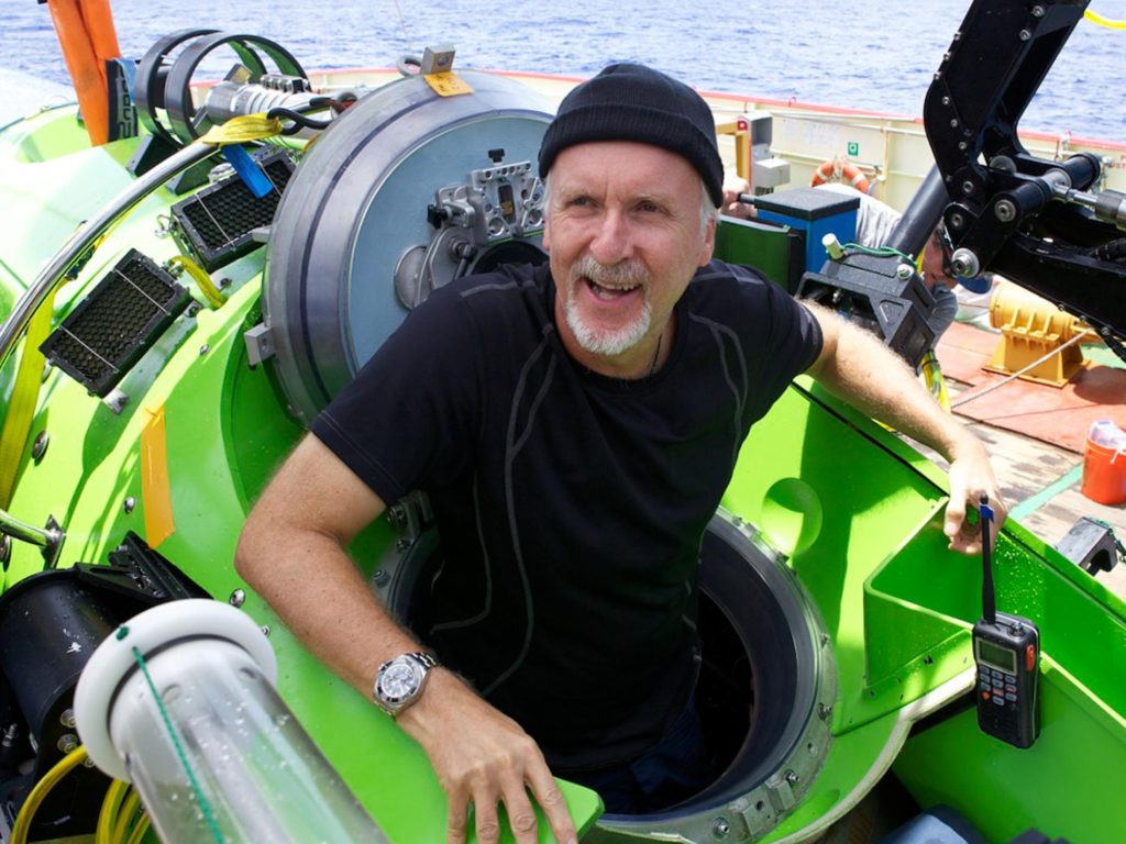
Artist’s concept drawing of Deepsea Challenger on the bottom. Source: http://divemagazine.co.ukDeepsea Challenger being lifted aboard its support vessel, the Mermaid Sapphire, after returning from the Challenger Deep. Source: National GeographicJames Cameron emerges from Deepsea Challenger after returning from the Challenger Deep. Source: National Geographic
A National Geographic film of his expedition, Deepsea Challenge 3D, was released to cinemas in 2012. You can watch the short movie trailer (2:44) here:
Cameron was awarded the 2013 Nierenberg Prize for Science in the Public Interest for his deep dive into the Challenger Deep. In the following long video (58:25) “Journey to the Deep,” he shares his experiences and perspectives from his record-setting dive.
The Deepsea Challenger is retired from diving.
2019: Victor Vescovo and the Five Deeps Expedition
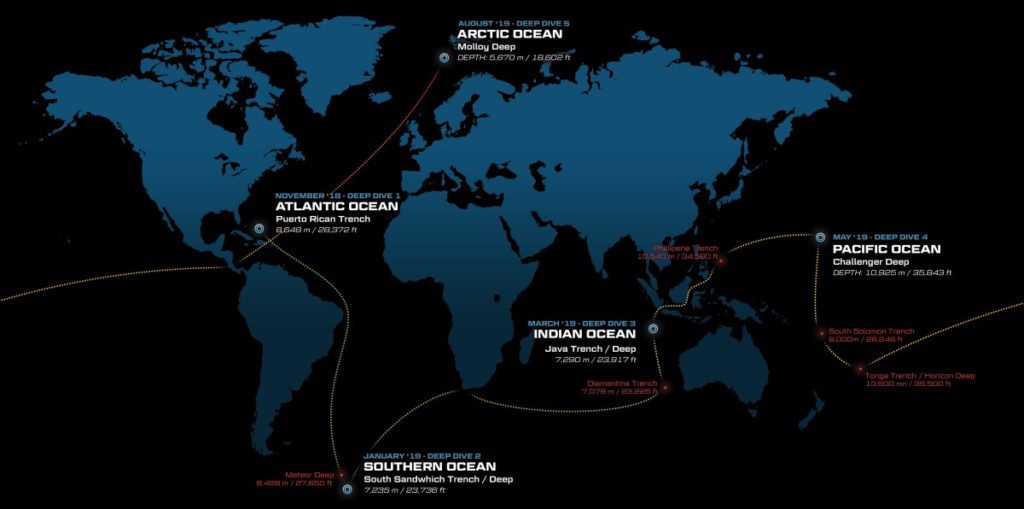
In 2015, businessman and explorer Victor Vescovo partnered with Triton Submarines LLC to design and build the two-person, 14-ton, titanium hull, deep-submergence vehicle Limiting Factor to enable Vescovo to conduct the Five Deeps Expedition to visit the deepest points in the world’s five oceans. The Five Deeps Expedition website is here:
During this period, the expedition covered 87,000 km (47,000 nautical miles) in 10 months and the Limiting Factor submersible completed 39 dives.
Locations of the Five Deeps diving sites. Source: https://tritonsubs.com/hadal/Victor Vescovo in full dive gear during his 2019 dives to the bottom of the Mariana Trench’s Challenger Deep. Source: Glenn Singleman photo via Wikipedia
The DSV Limiting Factor is a Triton 36000/2 submersible that is designed for dives to 11,000 m / 36,000 ft and pressure tested to 14,000 m / 45,991 ft. Like James Cameron’s Deepsea Challenger, the Limiting Factor is constructed with glass-bead based syntactic foam, which is very durable and able to withstand the enormous pressure placed on the submersible as it descends thousands of meters into the sea, and does so repeatedly without significant deformation or stress fractures developing over time.
The Limiting Factor has a Kraft Telerobotics “Raptor” hydraulic manipulator capable of functioning at full-ocean depth. Mission endurance is 16 hours plus 96 hours of emergency life support.
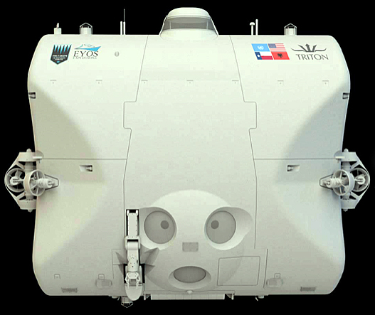
Triton 36000/2 exterior view. Access hatch is at the top center. Thrusters are located on the sides. View ports for the two-person crew are at the bottom center. Source: Five Deeps Expedition
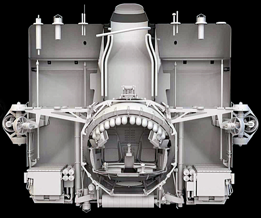
Triton 36000/2 interior view. The spherical titanium pressure vessel for the two-person crew sphere in the center, beneath the access trunk. Thrusters and their support structures are mounted to the pressure vessel. Source: Five Deeps Expedition
Using a Kongsberg EM124 multi-beam echo sounder mounted to the hull of the support vessel DSSV Pressure Drop, the Five Deeps Expedition team created detailed topographical maps of the Challenger Deep before the first of four dives. Dives 1 and 2 were conducted by Vescovo into the Eastern Pool. Dives 3 and 4 were conducted by Triton Submarines President, Patrick Lahey; Dive 3 was into the Eastern Pool and Dive 4 was into the Central Pool. Two days later, Dive 5 was conducted in the Sirena Deep. These five dives were accomplished in eight days. A synopsis of each dive follows:
Dive 1 (28 April 2019): This was the deepest dive of the mission and the deepest dive in human history. Vescovo reached the bottom at a depth of 10,925 meters ± 6.5 m (35,843 ft ± 21 ft, 10.92 km, 6.79 miles). Time on the bottom was 248 minutes. Note that the maximum depth originally was reported as 10,928 meters ± 10.5 meters, but this was later corrected. See the depth certification here: https://fivedeeps.com/wp-content/uploads/2019/10/Triton-LF-Max-Depth-Confirmation-for-Dives-12-DNV-GL.pdf
Dive 2 (3 May 2019): Vescovo reached a depth of 10,927 meters. Time on the bottom was 217 minutes.
Dive 3 (3 May 2019): This was a commercial certification dive with Patrick Lahey piloting and Jonathan Struwe aboard as a specialist. A Five Deeps Expedition scientific lander that became stuck on bottom during Dive 2 was freed from the bottom and recovered from 10,927 meters by direct action of the manned submersible (deepest salvage operation ever). Time on the bottom was 163 minutes. The submarine passed all of its qualification tests and commercial certification by DNV GL was granted following this dive.
Dive 4 (5 May 1959): This was a scientific dive with Patrick Lahey piloting and John Ramsay (the submarine’s designer) in the second seat. Video surveys were conducted and biological samples were collected. Time on the bottom was 184 minutes.
Dive 5 (7 May 2019): While still in the Mariana Trench area, Lahey conducted the first ever dive into the Sirena Deep, 128 miles (206 km) northeast of the Challenger Deep. On this dive (Dive 5), he reached a depth of 10,714 meters (35,151 ft, 6.66 miles). Time on the bottom was 176 minutes.
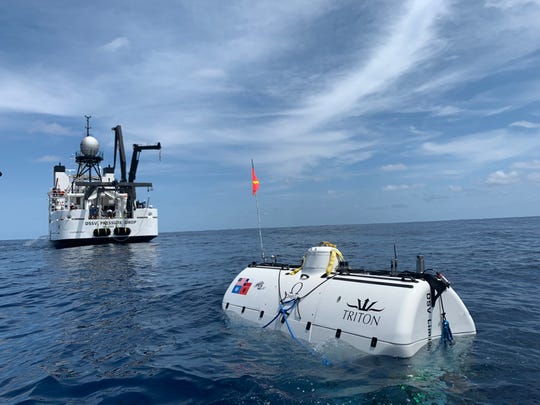
DSV Limiting Factor preparing to dive into the Challenger Deep Source: Triton Submarines LLC
DSV Limiting Factor being recovered by its support ship DSSV Pressure Drop. Source: Five Deeps Expedition
You’ll find a good summary of the five dives in the Challenger Deep and Sirena Deep in the expedition’s press release dated 13 May 2019, “Deepest Submarine Dive in History, Five Deeps Expedition Conquers Challenger Deep,” which is available here:
The entire expedition was filmed by Atlantic Productions for a five-part Discovery Channel documentary series, “Deep Planet.”
Into the future
The Triton 36000/2 Limiting Factor is the only submersible that is commercially certified for repeated exploration to the deepest points in the ocean. It is the only insurable, full ocean depth (FOD) manned submersible in the world. The official certification of the vessel to FOD is overseen by an independent third party, the world-standard credentialer of maritime vessels DNV-GL (Det Norske Veritas Germanischer Lloyd).
The manufacturer, Triton Submarines LLC, located in Vero Beach, Florida reported:
“Designed and certified to make thousands of dives to Hadal depths, during decades of service, Triton is excited to offer the opportunity for a private individual, government or philanthropic organization or research institute to acquire this remarkable System and continue the adventure.”
“Available to purchase today for $48.7 million, the Triton 36,000/2 Hadal Exploration System will be ready for delivery in 2019, after its successful (Five Deeps) expedition. The System will be fully proven. It will have extended the boundaries of human endeavor and technology. And it will offer a unique deep-diving capability unmatched by any nation or organization in the world.”
From space, Antarctica gives the appearance of a large, ice-covered continental land mass surrounded by the Southern Ocean. The satellite photo mosaic, below, reinforces that illusion. Very little ice-free rock is visible, and it’s hard to distinguish between the continental ice sheet and ice shelves that extend into the sea.
The following topographical map presents the surface of Antarctica in more detail, and shows the many ice shelves (in grey) that extend beyond the actual coastline and into the sea. The surface contour lines on the map are at 500 meter (1,640 ft) intervals.
Map of Antarctica and the Southern Ocean showing the topography of Antarctica (as blue lines), research stations of the United States and the United Kingdom (in red text), ice-free rock areas (in brown), ice shelves (in gray) and names of the major ocean water bodies (in blue uppercase text). Source: LIMA Project (Landsat Image Mosaic of Antarctica) via Wikipedia
The highest elevation of the ice sheet is 4,093 m (13,428 ft) at Dome Argus (aka Dome A), which is located in the East Antarctic Ice Sheet, about 1,200 kilometers (746 miles) inland. The highest land elevation in Antarctica is Mount Vinson, which reaches 4,892 meters (16,050 ft) on the north part of a larger mountain range known as Vinson Massif, near the base of the Antarctic Peninsula. This topographical map does not provide information on the continental bed that underlies the massive ice sheets.
A look at the bedrock under the ice sheets: Bedmap2 and BedMachine
In 2001, the British Antarctic Survey (BAS) released a topographical map of the bedrock that underlies the Antarctic ice sheets and the coastal seabed derived from data collected by international consortia of scientists since the 1950s. The resulting dataset was called BEDMAP1.
In a 2013 paper, P. Fretwell, et al. (a very big team of co-authors), published the paper, “Bedmap2: Improved ice bed, surface and thickness datasets for Antarctica,” which included the following bed elevation map, with bed elevations color coded as indicated in the scale on the left. As you can see, large portions of the Antarctic “continental” bedrock are below sea level.
Bedmap2 bed elevation grid. Source: Fretwell 2013, Fig. 9
For an introduction to Antarctic ice sheet thickness, ice flows, and the topography of the underlying bedrock, please watch the following short (1:51) 2013 video, “Antarctic Bedrock,” by the National Aeronautics and Space Administration’s (NASA’s) Scientific Visualization Studio:
NASA explained:
“In 2013, BAS released an update of the topographic dataset called BEDMAP2 that incorporates twenty-five million measurements taken over the past two decades from the ground, air and space.”
“The topography of the bedrock under the Antarctic Ice Sheet is critical to understanding the dynamic motion of the ice sheet, its thickness and its influence on the surrounding ocean and global climate. This visualization compares the new BEDMAP2 dataset, released in 2013, to the original BEDMAP1 dataset, released in 2001, showing the improvements in resolution and coverage. This visualization highlights the contribution that NASA’s mission Operation IceBridge made to this important dataset.”
On 12 December 2019, a University of California Irvine (UCI)-led team of glaciologists unveiled the most accurate portrait yet of the contours of the land beneath Antarctica’s ice sheet. The new topographic map, named “BedMachine Antarctica,” is shown below.
BedMachine Antarctica topographical map showing the underlying ground features and the large portions of the continental bed that are below sea level. Credit: Mathieu Morlighem / UCI
UCI reported:
“The new Antarctic bed topography product was constructed using ice thickness data from 19 different research institutes dating back to 1967, encompassing nearly a million line-miles of radar soundings. In addition, BedMachine’s creators utilized ice shelf bathymetry measurements from NASA’s Operation IceBridge campaigns, as well as ice flow velocity and seismic information, where available. Some of this same data has been employed in other topography mapping projects, yielding similar results when viewed broadly.”
“By basing its results on ice surface velocity in addition to ice thickness data from radar soundings, BedMachine is able to present a more accurate, high-resolution depiction of the bed topography. This methodology has been successfully employed in Greenland in recent years, transforming cryosphere researchers’ understanding of ice dynamics, ocean circulation and the mechanisms of glacier retreat.”
“BedMachine relies on the fundamental physics-based method of mass conservation to discern what lies between the radar sounding lines, utilizing highly detailed information on ice flow motion that dictates how ice moves around the varied contours of the bed.”
The net result is a much higher resolution topographical map of the bedrock that underlies the Antarctic ice sheets. The authors note:“This transformative description of bed topography redefines the high- and lower-risk sectors for rapid sea level rise from Antarctica; it will also significantly impact model projections of sea level rise from Antarctica in the coming centuries.”
You can take a visual tour of BedMachine’s high-precision model of Antarctic’s ice bed topography here. Enjoy your trip.
There is significant geothermal heating under parts of Antarctica’s bedrock
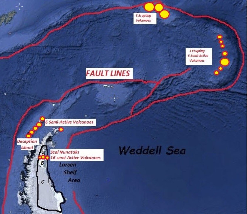
West Antarctica and the Antarctic Peninsula form a connected rift / fault zone that includes about 60 active and semi-active volcanoes, which are shown as red dots in the following map.
Volcanoes located along the branching West Antarctic Fault/Rift System. Source: James Kamis, Plate Climatology, 4 July 2017
In a 29 June 2018 article on the Plate Climatology website, author James Kamis presents evidence that the fault / rift system underlying West Antarctica generates a significant geothermal heat flow into the bedrock and is the source of volcanic eruptions and sub-glacial volcanic activity in the region. The heat flow into the bedrock and the observed volcanic activity both contribute to the glacial melting observed in the region. You can read this article here:
The correlation between the locations of the West Antarctic volcanoes and the regions of higher heat flux within the fault / rift system are evident in the following map, which was developed in 2017 by a multi-national team.
Geothermal heat flux distribution at the ice-rock interface superimposed on subglacial topography. Source: Martos, et al., Geophysical Research Letter 10.1002/2017GL075609, 30 Nov 2017
The authors note: “Direct observations of heat flux are difficult to obtain in Antarctica, and until now continent-wide heat flux maps have only been derived from low-resolution satellite magnetic and seismological data. We present a high-resolution heat flux map and associated uncertainty derived from spectral analysis of the most advanced continental compilation of airborne magnetic data. …. Our high-resolution heat flux map and its uncertainty distribution provide an important new boundary condition to be used in studies on future subglacial hydrology, ice sheet dynamics, and sea level change.” This Geophysical Research Letter is available here:
The results of six Antarctic heat flux models developed from 2004 to 2017 were compared by Brice Van Liefferinge in his 2018 PhD thesis. His results, shown below, are presented on the Cryosphere Sciences website of the European Sciences Union (EGU).
Spatial distributions of geothermal heat flux: (A) Pollard et al. (2005) constant values, (B) Shapiro and Ritzwoller (2004): seismic model, (C) Fox Maule et al. (2005): magnetic measurements, (D) Purucker (2013): magnetic measurements, (E) An et al. (2015): seismic model and (F) Martos et al. (2017): high resolution magnetic measurements. Source: Brice Van Liefferinge (2018) PhD Thesis.
Regarding his comparison of Antarctic heat flux models, Van Liefferinge reported:
“As a result, we know that the geology determines the magnitude of the geothermal heat flux and the geology is not homogeneous underneath the Antarctic Ice Sheet: West Antarctica and East Antarctica are significantly distinct in their crustal rock formation processes and ages.”
“To sum up, although all geothermal heat flux data sets agree on continent scales (with higher values under the West Antarctic ice sheet and lower values under East Antarctica), there is a lot of variability in the predicted geothermal heat flux from one data set to the next on smaller scales. A lot of work remains to be done …”
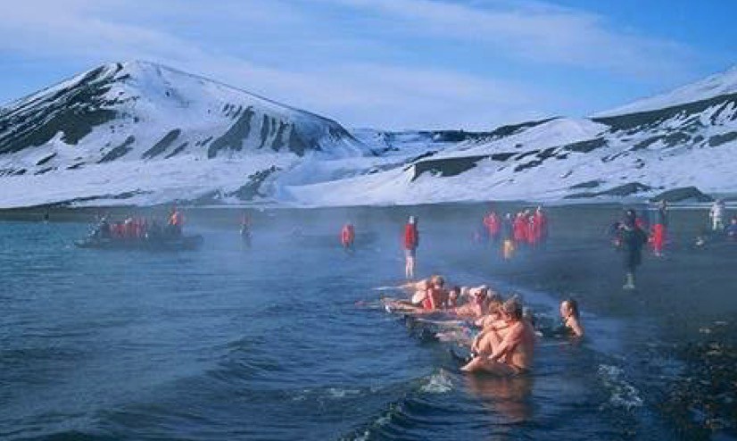
The effects of geothermal heating are particularly noticeable at Deception Island, which is part of a collapsed and still active volcanic crater near the tip of the Antarctic Peninsula. This high heat flow volcano is in the same major fault zone as the rapidly melting / breaking-up Larsen Ice Shelf. The following map shows the faults and volcanoes in this region.
Key geological features in the Larsen “C” sea ice segment area. Source: James Kamis, Plate Climatology, 4 July 2017Tourists enjoying the geothermally heated ocean water at Deception Island. Source: Public domain
So, if you take a cruise to Antarctica and the Cruise Director offers a “polar bear” plunge, I suggest that you wait until the ship arrives at Deception Island. Remember, this warm water is not due to climate change. You’re in a volcano.
Morlighem, M., Rignot, E., Binder, T. et al. “Deep glacial troughs and stabilizing ridges unveiled beneath the margins of the Antarctic ice sheet,” Nature Geoscience (2019) doi:10.1038/s41561-019-0510-8: https://www.nature.com/articles/s41561-019-0510-8
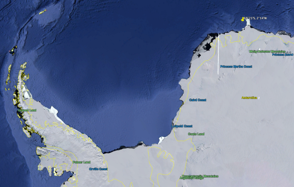
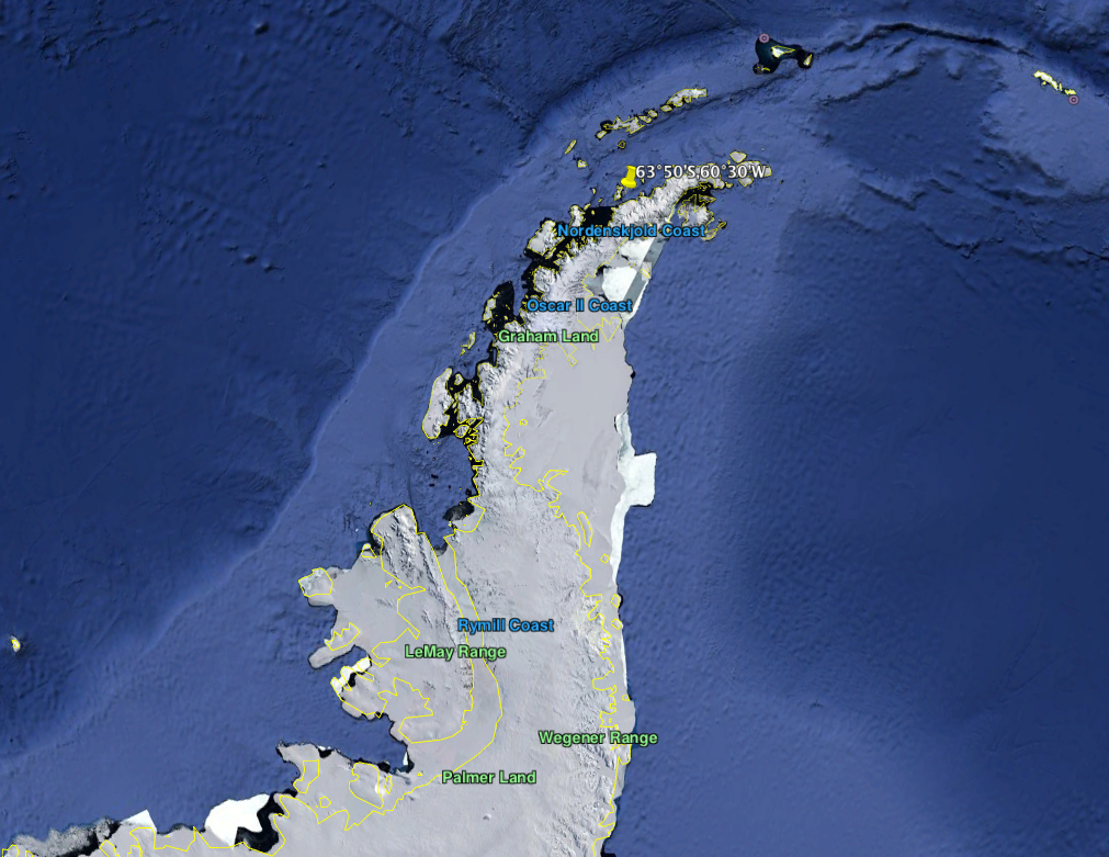
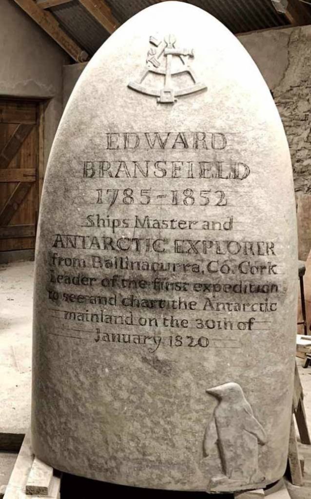
During his second voyage in 1773, British Captain James Cook became the first to cross the Antarctic Circle, but he was turned back by heavy sea ice without ever sighting the coast of Antarctica. It took 47 years before a Russian expedition, led by Estonian Fabien von Bellingshausen, sighted the coast of Antarctica. As the expedition leader, Bellingshausen generally is credited with the discovery of Antarctica on 28 January 1820. Just two days later, on 30 January 1820, a British expedition to the South Shetland Islands, led by Irish Lieutenant Edward Bransfield, sighted the tip of the Antarctic Peninsula. Bransfield is credited by some with the discovery of Antarctica. In this post, we’ll take a look at the voyages of these three pioneering Antarctic explorers.
Map of Antarctica and the Southern Ocean showing the topography of Antarctica (as blue lines), research stations of the United States and the United Kingdom (in red text), ice-free rock areas (in brown), ice shelves (in gray) and names of the major ocean water bodies (in blue uppercase text). Source: adapted from LIMA Project (Landsat Image Mosaic of Antarctica) via Wikipedia
Captain James Cook – First crossing of the Antarctic Circle, 17 January 1773
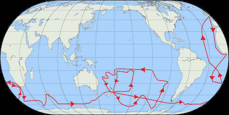
Setting out on their second voyage from England in July 1772, Captain James Cook (1728-1779) and his crew, on His Majesty’s Ship Resolution, circumnavigated the globe travelling as far south as possible to determine whether there actually was a great southern continent. The route covered during this voyage is shown in the following map.
Route of James Cook’s second voyage. Source: Jon Platek via Wikipedia
On 17 January 1773, Cook made the first recorded crossing of the Antarctic Circle, which he reported in his log:
“At about a quarter past 11 o’clock we cross’d the Antarctic Circle, for at Noon we were by observation four miles and a half south of it and are undoubtedly the first and only ship that ever cross’d that line.”
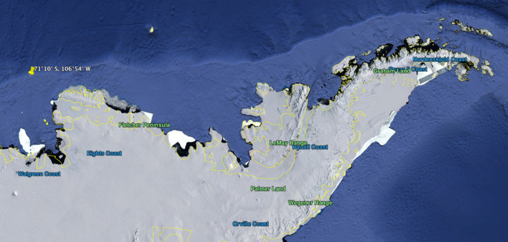
Cook crossed the Antarctic Circle three times during his second voyage. The last crossing, on 30 January 1773, was to be the most southerly penetration of Antarctic waters, reaching latitude 71°10’ S, longitude 106°54’ W. The ship was forced back due to solid sea ice. Cook came within about 240 km (150 mi) of the Antarctic mainland on his second voyage.
Cook’s southernmost approach to Antarctica (yellow pin, left). Source: Google Earth
Fabien von Bellingshausen – First sighting of Antarctica, 28 January 1820
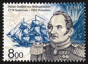
In 1818, the Russian Empire, ruled by Czar Alexander I, organized two expeditions to study the polar regions, one for mapping the Arctic and one for sailing further south than Captain James Cook’s second voyage 45 years earlier. The southern polar expedition was led by the prominent cartographer Fabien Gottlieb Benjamin von Bellingshausen, who was born in 1778 on Saaremaa, the largest island in today’s Republic of Estonia. This was to became known as the Bellingshausen Expedition.
The expedition consisted of two ships, Bellingshausen’s 985 ton flagship sloop Vostok, and the 530 ton support sloop Mirnyi, under the command of Mikhail Lazarev (Bellingshausen’s second-in-command). An exhibit at the Estonian Maritime Museum in Tallinn reported: “The largest proportion (a whopping 65.8 tons) of the food stock on the Bellingshausen expedition consisted of wheat and rye cookies. In addition, they brought 28 tons of salted meat and 20.5 tons of dried peas. In ports, the crew also acquired cereal and fresh food.” In Antarctic waters, icebergs would supply their fresh water needs.
On 4 June 1819, the expedition departed from the Russian naval island base at Kronstadt, just off the coast from Saint Petersburg. Seven months later, the expedition crossed the Antarctic Circle on 26 January 1820.
The Bellingshausen expedition is credited with being the first to reach Antarctica on 28 January 1820, when the two ships approached to within 20 miles (32 km) of the Antarctic coast, at latitude 69°21’28” S, longitude 2°14’50” W, in an area now known as Princess Martha Coast in East Antarctica. Bellingshausen reported sighting an ice shelf that today is known as the Fimbul ice shelf.
Location of Bellingshausen’s first sighting of Antarctica on 28 January 1820 (yellow pin, upper right). Source: Google Earth
Bellingshausen did not claim to have discovered Antarctica, but his descriptions of what he saw agree very well with what the Princess Martha Coast is now known to look like. On the basis of this sighting and the coordinates given in his log book, Bellingshausen generally is credited (e.g., the British polar historian A. G. E. Jones) with the discovery of the Antarctic continent.
In their subsequent circumnavigation of the Antarctic continent, Bellingshausen and Lazarev became the first explorers to see and officially discover several parts of the Antarctic landmass. On 22 February 1820, the Vostok and Mirnyi were hit by the worst storm of the voyage and were forced to sail north, arriving in Sydney, Australia in April. After several months exploring the South Pacific and then hearing about the sighting of Antarctica by the British (Edward Bransfield and William Smith), the Bellingshausen Expedition sailed from Sydney on 11 November 1820 to continue exploring the Antarctic. On 24 December 1820, the two ships once again were south of the Antarctic Circle. On this part of the voyage, Bellingshausen discovered and named Peter I Island and the Alexander Coast, now known as Alexander Island, along the west coast of the Antarctic Peninsula.
The circumnavigation route followed by the Bellingshausen Expedition is shown in the following map. Bellingshausen became only the second explorer, after Cook, to have circumnavigated Antarctica.
Route map of the Bellingshausen Expedition to Antarctica: 1819-21. Source: Bourrichon via Wikipedia
The Bellingshausen expedition returned to Kronstadt on 4 August 1821, ending a voyage that had lasted two years and 21 days and covered about 50,000 miles (80,467 km). After his return, Bellingshausen was promoted to the rank of Admiral and Lazarev was promoted to the rank of Lieutenant–Captain. His travel account was not published until ten years later.
As part of the International Geophysical Year (IGY) in the mid-1950s, the Soviet Union established its first two Antarctic bases, which were named Mirnyi (established 13 February 1956) and Vostok (established 6 December 1957), in honor of the ships in the Bellingshausen Expedition.
2003 Estonian stamp commemorating Bellingshausen’s discovery of Antarctica. Source: eBay
The Bellingshausen expedition was commemorated on a 2003 Estonian stamp that features a portrait of Bellingshausen and a drawing of his flagship Vostok over a map showing the route of his Antarctic expedition.
Edward Bransfield – Sighting of Antarctica, 30 January 1820
In February 1819, British merchant ship owner William Smith, aboard his vessel The Williams, was sailing from Buenos Aires, Argentina to Valparaiso, Chile. To catch the prevailing winds, he sailed unusually far south of Cape Horn and, on 19 February 1819, sighted previously unknown islands in the Southern Ocean. To confirm his sighting and to chart the islands, Royal Navy officials in Valpariso chartered his ship and assigned Sailing Master Lieutenant Edward Bransfield, from Ballinacurra, Ireland (near Cork), to accompany Smith on an expedition back to the islands, which would become known as the South Shetland Islands. During this expedition, Bransfield landed on King George Island and took formal possession on behalf of King George III.
On 30 January 1820, Bransfield sighted the Trinity Peninsula, which is the northernmost tip of the Antarctic Peninsula. His sighting was made at about latitude 63°50’S and longitude 60°30’W.
Location of Bransfield’s first sighting of Antarctica (yellow pin, top center) on 30 January 1820. Source: Google Earth
After the initial sighting, Bransfield charted a segment of the Trinity Peninsula and followed the edge of the ice sheet in a north-easterly direction, where he discovered various points on Elephant Island and Clarence Island, which he formally claimed for the British Crown. In his log, Bransfield made a note of two “high mountains, covered with snow”, one of which subsequently was named Mount Bransfield in his honor. The Bransfield Strait between the South Shetland Islands and the Antarctic Peninsula also was named in his honor in 1822 by Antarctic explorer James Weddell.
Since Bransfield’s sighting, the tip of the Antarctic Peninsula has been known variously as Trinity Land, Palmer Land, Graham Land, and Land of Louis Philippe. Prime Head is the northernmost point of this peninsula.
Bransfield’s expedition charts were given to the Admirality and currently are in the possession of the UK Hydrographic department in Taunton, Somerset.
In 2000, Bransfield’s historic achievement was recognized when the Royal Mail issued a stamp in his honor. Since no likeness of the man survives, the stamp depicted an image of the RRS Bransfield, a British Antarctic surveying vessel.
2000 Royal Mail commemorative stamp. Source: Commonwealth Stamps Opinion
To commemorate the 200th anniversary of Edward Bransfield’s sighting of Antarctica (and some say, his discovery of Antarctica), a memorial by sculptor Matt Thompson will be erected in Ballinacurra, Ireland in January 2020.
Edward Bransfield memorial, work in progress. Source: Tony Whelan photo, Afloat.ie
Estonia’s Antarktika 200 expedition
To commemorate the 200th anniversary of the discovery of Antarctica by the Bellingshausen Expedition, the Estonian Maritime Museum and NGO Thetis Expeditions have organized a scientific expedition from Kronstadt, Russia to the Antarctic peninsula by a crew of 12 aboard the 24 meter, 95 ton, Estonian-registered sailing yacht S/Y Admiral Bellingshausen.
The planned route, which includes about 50 stops, and approximately follows the Bellingshausen’s route to and from the Southern Ocean, is shown in the following map. The crew will take samples of pollen, water and microplastics while on the voyage, for researchers at Estonia’s University of Tartu. The expedition includes food of Estonian origin to the largest possible extent, and probably a better selection of food than on Bellingshausen’s 1819 – 1821 voyage.
Antarktika 200 route map. Source: International Maritime Rescue Federation
The ship departed Tallinn harbor on 14 July 2019, and headed for its first port of call at the historic Russian naval island base at Kronstadt, which was the starting point for the Bellingshausen Expedition.
You can follow the current position on the S/Y Admiral Bellingham at the following link:
On 3 January 2020, the ship was moored in Ushuaia, Argentina, in preparation for its voyage across the Drake Passage to Antarctica. The ship is scheduled to reach Antarctica in time to celebrate the 200th anniversary of Bellingshausen’s discovery on 28 January 2020.
This voyage will be the subject of a TV documentary. For more information on the Antarktika 200 expedition, visit the following website:
Best wishes to the crew of S/Y Admiral Bellingshausen for a safe and successful voyage.
Composite map of early expeditions in Antarctic waters
The following map provides a good overview of the routes taken by the early Antarctic explorers, none of whom went ashore.
Source: Antarctic Logistics
The first landings in Antarctica
An unconfirmed first landing at Hughes Bay, on the northwest coast of the Antarctic Peninsula, may have been made on 7 February 1821 by Captain John Davis and crew members from the American sealing ship Cecilia, which had been sailing in the vicinity of the South Shetland Islands in search of seals. The ship’s log recorded that men were ashore to look for seals at latitude 64°01’S. The logbook entry concluded with the statement, “I think this Southern Land to be a Continent.”
The first substantiated landing in Antarctica was not made until 74 years later, on 24 January 1895, when seven men from the Norwegian whaling and sealing ship Antarctic, came ashore in the vicinity of Cape Adare, on the Ross Sea almost due south of New Zealand. New Zealander Alexander Francis Henry von Tunzelmann is sometimes credited as being the first person to set foot on the Antarctic mainland.
For more information on Fabien Bellingshausen & Mikhail Lazarev
The birthdate of Isaac Asimov, a famous author best known for his science fiction novels and short stories, is sometime between 4 October 1919 and 2 January 1920. He was born in Petrovichi in Smolensk Oblast, RSFSR (now Russia), west of Moscow, near the border with Belarus, and he died in New York City on 6 April 1992. He traditionally celebrated his birthday on 2 January, giving enough reason to mark the centennial of his birth on 2 January 2020.
You’ll find short biographies of Isaac Asimov at the following links:
Left: Isaac Asimov circa 1959 (Wikipedia) Right: Asimov circa 1980s (Goodreads.com)
I was an avid reader of science fiction during the time when Isaac Asimov’s novels on robots, the Foundation and the Galactic Empire were first being published. I was hooked with the first novel I read, Pebble in the Sky, and waited with anticipation until each new book became available in paperback.
You may remember that Asimov created the basic three laws of robotics:
A robot may not injure a human being or, through inaction, allow a human being to come to harm.
A robot must obey the orders given it by human beings except where such orders would conflict with the First Law.
A robot must protect its own existence as long as such protection does not conflict with the First or Second Laws.
These laws were woven into the storyline of many of his books.
Unless you already have your favorite Asimov volumes on your bookshelf, I suggest that you visit the Internet Archive and the Open Library, which provide free access to many Asimov books as well as a vast range of other books and resources. You can set up a free account on the Internet Archive homepage here:
The Open Library contains many of his books and other books about him, all of which you can borrow as e-books for two weeks. You can navigate to the Open Library from the Internet Archive home page or use the following direct link: https://openlibrary.org
In the Open Library, a search for “Isaac Asimov” will take you here:
Now you’re almost ready to look for an available book in the Open Library and start reading. Note that you may be in a waitlist, because library rules for e-books limit the number of copies that can be checked out at any one time.
If you choose to read about robots, the Foundation and the Galactic Empire (books written over a 52 year period from 1940 to 1992), consider Asimov’s own recommendations regarding the chronological order of the stories, in terms of future history:
The Complete Robot (1982). This is a collection of 31 robot short stories published between 1940 and 1976 and includes every story in Asimov’s earlier collection: I, Robot (1950).
The Positronic Man (1992): A stand-alone robot novel set from the 22nd to 24th centuries, co-written with Robert Silverberg, based on Asimov’s 1976 novelette “The Bicentennial Man”
Nemesis (1989): A standalone novel, set in the 23rd century in a star system about 2 light years from Earth, when interstellar travel was new
Caves of Steel (1954). This is the 1st robot novel.
The Naked Sun (1957). This is the 2nd robot novel.
The Robots of Dawn (1983). This is the 3rd robot novel.
Robots and Empire (1985). This is the 4th robot novel.
The Currents of Space (1952). This is the 1st Empire novel.
The Stars, Like Dust (1951). This is the 2nd Empire novel.
Pebble in the Sky (1950). This was Asimov’s first novel. It is the 3rd Empire novel.
Prelude to Foundation (1988): This is the 1st Foundation novel, actually a prequel.
Forward the Foundation (1992): Published posthumously, this is the 2nd Foundation novel, and the 2nd prequel.
Foundation (1951). This is the 3rd Foundation novel. It is a collection of four stories published between 1942 and 1944, plus an introductory section written in 1949.
Foundation and Empire (1952). This is the 4th Foundation novel. It is made up of two stories originally published in 1945.
Second Foundation (1953): This is the 5th Foundation novel. It is made up of two stories originally published in 1948 and 1949.
Foundation’s Edge (1982): This is the 6th Empire novel.
Foundation and Earth (1986): This is the 7th Empire novel.
The End of Eternity (1955): A standalone novel, about Eternity, an organization “outside time” which aims to improve human happiness by altering history.
The above list is adapted and updated from the Author’s notes in Prelude to Foundation to account for books published after 1988.
I also recommend that you take the time to watch the following on YouTube:
Isaac Asimov – The Last Question (28.06 minutes). This is one of Asimov’s best-known and most acclaimed short stories, published in 1951. Presented as a narration on YouTube: https://www.youtube.com/watch?v=ojEq-tTjcc0
Nightfall by Isaac Asimov – X Minus One (26:49 minutes): One of Asimov’s earliest short stories, published in 1941. This is a story about an inhabited planet with multiple suns. Presented as a narration on YouTube: https://www.youtube.com/watch?v=aRJO4dYZ4NQ
In a 12 December 2019 NUCNET article, David Dalton, reporting on the United Nations Framework Convention on Climate Change (COP25) in Madrid, summarized the following points made by International Atomic Energy Agency (IAEA) director-general Rafael Mariano Grossi:
The world is “well off the mark” from reaching the climate goals of the Paris Agreement.
Around two-thirds of the world’s electricity still is generated through burning fossil fuels.
Greater use of low-carbon nuclear power is needed to ensure the global transition to clean energy includes a baseload backup to variable renewable energy sources such as solar and wind.
Greater deployment of a diverse mix of low-carbon sources such as hydro, wind and solar, as well as nuclear power, and battery storage, will be needed to reverse that trend and set the world on track to meet climate goals.
I concur with these points and feel that Mr. Grossi has laid out a reasonable and responsible position on the future role of nuclear power in “green” energy solutions that are focused on the primary goal of reducing worldwide carbon dioxide emissions. The commercial nuclear power industry has demonstrated the ability to reliably generate carbon-free electricity, 24 hours a day, seven days a week, in units of a thousand megawatts or more per power plant. Except for the largest hydroelectric facilities, no other component of a carbon-neutral energy infrastructure offers such capabilities, which are essential for delivering 24/7 service to large users and stabilizing the grid. Unfortunately, Mr. Grossi’s view is not shared by many EU energy advocates seeking to get member states to agree to the EU “Green Deal.”
The Energy Union has quite a challenge, starting with the EU’s energy mix (circa 2016) as shown in the following chart:
EU 2016 energy mix. Source: EU Statistical Pocketbook 2018
Complicating matters, the EU currently imports nearly 40% of its natural gas from Russia.
The European Union’s Green Deal is described as “a new growth strategy that aims to transform the EU into a fair and prosperous society, with a modern, resource-efficient and competitive economy where there are no net emissions of greenhouse gases in 2050 and where economic growth is decoupled from resource use.” You’ll find the EU’s 11 December 2019 detailed description of the Green Deal here: https://eur-lex.europa.eu/legal-content/EN/TXT/?qid=1576150542719&uri=COM%3A2019%3A640%3AFIN
To enforce this “Green Deal,” the EU intends to adopt a “climate law” that is scheduled to be presented to Member States in March 2020.
The EU’s “Green Deal” is strongly biased against almost anything except renewable energy sources
On 11 December 2019, Reuters reported that, “European Union states have blocked a set of new rules governing which financial products can be called ‘green’ and ‘sustainable’, EU officials said, in a major setback for the bloc’s climate ambitions.” The Reuters report noted that EU lawmakers wanted nuclear and fossil fuel funding clearly excluded from the definition of “green” investments. You can read this Reuters report here: https://af.reuters.com/article/commoditiesNews/idAFL8N28L3GD
This EU position is a particular problem for France, where nuclear power provided 71.7% of total French generating capacity in 2018 and about 90% of total electrical capacity was provided by low-carbon sources (nuclear + renewables). In October 2019, Électricité de France announced that it is planning to make a decision in 2021 on building several more large nuclear power plants, which will be needed in the next decade as its oldest 900 MWe pressurized water reactor (PWR) plants start reaching their retirement age.
In contrast, nuclear power provided 11.8% of total German generating capacity in 2018 and about 47% of total electrical capacity was provided by low-carbon sources (nuclear + renewables), while 48.3% of total generating capacity was provided by a fossil fuel sources. Germany plans to decommission the last of its seven remaining nuclear power plants, representing an aggregate of 9,256 MWe of carbon-free electric generating capacity, in the next three years, by December 2022. It will be a challenge for new renewable energy sources to be deployed in time to make up for the lost carbon-free generating capacity from nuclear power. It is notable that Germany gets 7% of its total generating capacity from burning biomass, which the EU, in its great wisdom, defines as a carbon-neutral renewable energy source. More on that later.
How does the EU define “clean energy”?
The EU’s definition of “clean energy” is rather elusive. On the EU Green Deal website, the Clean Energy fact sheet identifies the following three “key principle:”
Prioritize energy efficiency and develop a power sector based largely on renewable sources
Secure and affordable EU energy supply
Fully integrated, interconnected and digitalized EU energy market
Only “renewable sources” are actually defined as sources for “clean energy.” Nuclear power is not identified as a “clean” energy source. I was unable to find on the EU Green Deal website any performance metrics related to “clean” energy source performance relative to carbon emissions.
Another EU description of “clean energy” can be found the “Clean Energy for all Europeans” program, which focuses on the following:
Energy efficiency first, focusing on energy saving opportunities and “smarter” / “greener” buildings.
More renewables, with a new target of at least 32% in renewable energy by 2030
Better governance of the Energy Union, including a new energy “rulebook” under which each EU Member State drafts a National Energy and Climate Plan (NECP)
More rights for consumers to produce, store or sell their own energy
The focus is on a distributed electric power infrastructure that takes advantage of many ways to improve energy efficiency, manage power consumption and generate power from distributed renewable energy sources. Nuclear power is not mentioned at all in this document. However, “large scale biopower” from agricultural and forest sources is addressed.
How does the EU define “renewable energy sources”?
The latest EU directive on the promotion of energy use from renewable sources is Directive (EU) 2018/2001, dated 11 December 2018. The definition of “renewable energy sources” traces back to Directive 2003/54/EC, dated 26 June 2003:
“Renewable energy sources” means renewable non-fossil energy sources (wind, solar, geothermal, wave, tidal, hydropower, biomass, landfill gas, sewage treatment plant gas and biogases)
So, fossil energy sources are excluded and nuclear energy sources are not included.
This seems logical but the devil is in the details. The main problem is that EU energy policy equates “renewable” with being “carbon free,” when, for some renewable energy sources, this is far from the truth. As an example, existing EU policy treats burning wood fuel in power plants as carbon-neutral while this fuel generates 15 to 20% more carbon dioxide per megawatt than the coal fuel it replaces. This has resulted in a trend among EU coal-burning power plants to switch to wood pellets and claim the emission credit while actually polluting more than before. See my 7 January 2017 post, “Hey, EU!! Wood may be a Renewable Energy Source, but it isn’t a Clean Energy Source,” for details. The direct link to this post is here: https://lynceans.org/all-posts/hey-eu-wood-may-be-a-renewable-energy-source-but-it-isnt-a-clean-energy-source/
Fortunately, this matter may be on its way to being addressed in an EU court. A 4 March 2019 article by Karen Savage, writing for Climate Liability News, reports, “The suit, which was filed in the European General Court in Luxembourg, asks the court to prevent EU countries from counting forest wood as a renewable energy source under the 2018 revised Renewable Energy Directive known as RED II.” Major sources of wood pellets used in EU power plants are in the southeast U.S., where greatly increased logging activities are depleting established, slow-growth hardwood forests. So the EU is OK with a “clean” energy policy that, in practice, increases current pollution locally in the EU while simultaneously stripping hardwood forests in a location outside of the EU. It seems to me that this is an environmental “double whammy” that can only make sense on paper, but not in practice. You can read Karen Savage’s article here: https://www.climateliabilitynews.org/2019/03/04/biomass-european-union-lawsuit/
Conclusions
Regarding the EU Green Deal and Energy Union, I’m certain that the devil is in the details, and EU Member States need to have the opportunity to assess these details so there is no misunderstanding when EU climate laws are passed.
The EU’s Green Deal has major flaws and needs to be recast to acknowledge the important role that nuclear power can play as a large, carbon-free source of electric power while also helping to ensure 24/7 grid stability. Failing to recognize the role of nuclear power as a carbon-free source of electric power will serve to highlight the strong bias and hypocrisy of an EU energy leadership that has lost its way. It also would serve as another example of why Brexit makes sense.
Even fossil power, with appropriate advanced environmental controls, should have a role in the Green Deal. For example, a rapid shift away from coal to natural gas would significantly decrease near-term carbon dioxide emissions. Similarly, abandoning the laughable EU policy on “carbon-neutral” biomass would eliminate a significant source of carbon dioxide emissions within the EU, and it would save environmentally valuable hardwood forests in the southeast U.S. and elsewhere.
Update: 16 December 2019 – Finally, some common sense prevailed, but only under very intense political pressure and, probably, fear of failure
In an article by Samuel Petrequin, “EU leaders include nuclear energy in green transition,” the Associated Press reported:
“EU heads of state and government agreed that nuclear energy will be recognized as a way to fight climate change as part of a deal that endorsed the climate target. While Poland did not immediately agree to the plan, the concessions on nuclear energy were enough for the Czech Republic and Hungary to give their approval. The two nations had the support of France, which relies on nuclear power for 60% of its electricity. They managed to break the resistance of skeptical countries, including Luxembourg, Austria and Germany to get a clear reference to nuclear power in the meeting’s conclusions. ‘Nuclear energy is clean energy,’ Czech Prime Minister Andrej Babiš said. ‘I don’t know why people have a problem with this.’”
The European Council memorandum contains only a single reference to “nuclear,” more in the form of a resigned acknowledgement rather than an endorsement.
“The European Council acknowledges the need to ensure energy security and to respect the right of the Member States to decide on their energy mix and to choose the most appropriate technologies. Some Member States have indicated that they use nuclear energy as part of their national energy mix.”
Congratulations to the representatives from France, Czech Republic, Hungary, Poland and others for fighting the hard political fight and winning a place for nuclear power in the EU’s Green Deal. But be watchful because the EU anti-nuclear forces are still there.
Update: 20 March 2020 – Yes, the EU anti-nuclear forces are still there.
On 10 March 2020 the European Commission issued a press release announcing its new industrial strategy, “Making Europe’s businesses future-ready: A new Industrial Strategy for a globally competitive, green and digital Europe.” You can read the press release and download related documents here: https://ec.europa.eu/commission/presscorner/detail/en/ip_20_416
While the plan highlights the need to “secure a sufficient and constant supply of low-carbon energy at competitive prices,” the word “nuclear” is notably absent from the EU’s industrial strategy. Not much of a surprise, considering the EU’s behavior on the Green New Deal.
The next day, on 11 March, the Brussels-based nuclear industry group Foratom called on the EU decision-makers to support the nuclear sector’s important role within the EU economy. Foratom’s Director General, Yves Desbazeille, noted, “Not only is it (nuclear) low-carbon, it is also flexible, dispatchable and cost-effective”.
Foratom highlighted the following key attributes of nuclear energy in the context of the EU industrial strategy:
Maintain the competitiveness of Europe’s industry as energy often accounts for a significant share of manufacturing costs,
Decarbonize industry and thus contribute towards the 2050 carbon neutrality target,
Provide industry with the energy it needs when it needs it, which is particularly important for processes which run 24/7,
Other industries by offering alternative sources of decarbonized energy such as hydrogen and heat (sector coupling).
This is further evidence that EU nuclear energy advocates are fighting an uphill battle for recognition by the entrenched EU bureaucracy that nuclear power is a zero-carbon source of power and it can make an important (and maybe essential) contribution to meeting the EU’s 2050 carbon neutrality goal.
Best wishes to Foratom in their efforts to secure a place in the EU industrial strategy for nuclear power.
Update 5 May 2020 – More support for EU nuclear power
SNETP (Sustainable Nuclear Energy Technology Platform) was established in 2007, with EC support, as a group of non-governmental organizations that promote and coordinate research on nuclear fission.
On 24 April 2020, SNETP sent a letter, endorsed by more than 100 organizations, to the Vice-presidents of the European Commission and the EU Commissioner for Energy calling for a “just and timely assessment of nuclear energy in the EU Taxonomy of Sustainable Finance.”
When enacted, the EU’sTaxonomy Regulation is intended to be a tool to guide future energy investments by providing investors with information on which activities and technologies contribute to the EU’s sustainability goals. In their March 2020 final recommendations, the technical expert group (TEG) currently advising the EC on sustainable energy finance did not include nuclear power as a low-carbon and sustainable electricity source.
Clearly, the battle lines have formed, with the anti-nuclear elements of the EU bureaucracy on one side and organizations like Foratom and SNETP on the other. Against the behemoth EU bureaucracy, my best wishes go out to the underdogs, Foratom, SNETP, and other organizations and individuals that understand how nuclear power can play important roles in helping the EU achieve climate neutrality by 2050.
My 11 December 2018 post, “Lots of Land Speed Record (LSR) Action in 2018,” provides background information on land speed record governance and a look at the fastest cars competing in the 2018 LSR season. 2018 highlights included:
The North American Eagle team, with driver Jessi Combs, continued to extend the performance of their jet-powered LSR car on a track in the Alvord Desert in Oregon.
The Bloodhound team in the UK was saved from insolvency, literally at the last moment, when the business and assets were bought by Yorkshire-based entrepreneur Ian Warhurst.
Salt conditions at the Bonneville salt flats in Utah were very good and many speed records were broken.
The North American Eagle LSR car crashed during a high-speed run in the Alvord Desert in August, killing driver Jessi Combs.
The salt conditions at the Bonneville salt flats were poor, resulting in rough driving conditions and generally lower speeds during Bonneville Speed Week (August) and the Utah Salt Flats Racing Association (USFRA) World of Speed (September). The Bonneville World Finals (October) were cancelled because of wet conditions.
The Carbinite LSR car, the Carbiliner, crashed during a high-speed run at the World of Speed 2019 in September, severely injuring driver Rob Freyvogel.
The 29th Annual Speed Week at Lake Gairdner, Australia in March had only one run over 300 mph (483 kph) in hot, dry conditions.
Now with proper financing, the Bloodhound LSR team transitioned to the next phase of the project, arriving at the Hakskeen Pan track in South Africa in October and conducting high-speed testing, which concluded successfully in November.
Let’s take a look at the 2019 LSR season in more detail.
1. North American Eagle
In August 2019, the North American Eagle team, with driver Jessi Combs, returned to the Alvord Desert in Oregon to attempt to break the official Women’s Land Speed Record set by Kitty O’Neil in 1976 with a two-way average speed of 512.710 mph (825.127 kph) in the rocket-powered SMI Motivator at the same venue. The North American Eagle team website is here: https://www.landspeed.com
The North American Eagle land speed record car. Source: North American EagleDriver Jessi Combs. Source: North American Eagle
An investigation into the cause of the crash revealed that the front wheel assembly of the car collapsed, possibly due to collision damage from hitting something on the track at high speed.
North American Eagle Crew Chief Les Holm reported Jessi Combs’ second run was measured at a speed of 548.342 mph (882.471 kph), yielding a two-way average speed of 531.889 mph (855.992 kph). Hemmings news reported that the North American Eagle team has submitted Jessi Combs’s two-way average speed results to the Guinness Book of World Records to claim the title of fastest woman on the planet.
It is not yet known if Jessi Combs’ two-way average speed will qualify as an official FIA world land speed record.
The Petersen Automotive Museum in Los Angeles held an exhibition entitled “Jessi Combs: Life at Full Speed” to commemorate the life and accomplishments of this extraordinary person.
Source: Petersen Automotive Museum
The Jessi Combs Foundation was founded in 2019. The mission of the Foundation is to “educate, inspire and empower the next generation of female trailblazers and stereotype-breakers.” The Foundation’s website is here: https://www.thejessicombsfoundation.com/mission-statement/
In June 2020, the Guinness World Record was posthumously awarded to Jessi Combs, declaring: “The fastest land speed record (female) is 841.338 kph (522.783 mph), and was achieved by Jessi Combs (USA) in the Alvord Desert, Oregon, USA, on 27 August 2019. Jessi is the first person to break this record in more than 40 years.” This record is posted on the Guinness World Records website here: https://www.guinnessworldrecords.com/world-records/fastest-land-speed-record-(female)
2. Bonneville Speed Week 2019: 13 – 15 August 2019
Now let’s look at a few of the top challengers at Speed Week 2019.
Turbinator II
At the Bonneville World Finals in 2018, Team Vesco’s gas turbine powered Turbinator II, with Dave Spangler driving, made a one-way run through the measured mile of 493.996 mph (795.009 kph), with an exit speed of 503.332 mph (810.034 kph). Turbinator II became the world’s first wheel-driven vehicle to exceed 500 mph and 800 kph.
In 2019, Dave Spangler was unable to complete a single run with Turbinator II during Bonneville Speed Week 2019. Three runs on the 2-mile “short” course were attempted on 14 – 15 August, but none were completed, for a variety of issues. You can watch a short video about Team Vesco at Speed Week 2019 here:
After Speed Week 2019, Team Vesco reported, “In the interest of safety and to correct our course while navigating toward our goal to become the first wheel driven car to set an official National or World record over 500 MPH, we must discontinue racing for the remainder of 2019. To improve our team, we have already begun a search for a company with turbine control engineering capabilities to partner with us.” You’ll find more information on the Team Vesco website here: https://www.teamvesco.com
Speed Demon
George Poteet’s Speed Demon is a blown (supercharged or turbocharged) fuel (not gasoline) streamliner (BFS) that currently holds two-way land-speed records in five out of seven of Bonneville’s BFS classes: A, B, C, D and F. The two remaining classes are AA/BFS and E/BFS. The team’s goals for 2019 were to achieve records in these remaining classes and to raise its fastest two-way speed record to over 480 mph (772 kph). The teams current record, set in 2013, stands 437.183 mph (703.578). You can read more about these plans in the following Motor Tend article: https://www.hotrod.com/articles/pottet-speed-demon-aims-480-mph-bonneville/
To compete in several different classes, Speed Demon is designed to accommodate several different displacement engines that have been configured to fit inside the car’s svelte fuselage. At Speed Week 2019, the team had four different Duttweiler engines to challenge BFS records in Classes A, AA, C and E.
Speed Demonwas the only car that made runs over 300 mph (483 kph) during Speed Week 2019. On the “long” course, which was shortened to two miles because of poor salt conditions, Speed Demon achieved the following speeds:
13 Aug 2019: 300.648 mph (483.846 kph) and 332.815 mph (535.614 kph) with the E “small block” engine
15 Aug 2019: 369.533 mph (594.706 kph) with the AA “big block” engine
None of these runs broke an existing class speed record. However, Speed Demon and George Poteet were honored with the Hot Rod Magazine trophy for fastest run during Speed Week 2019.
Tom Flattery’s Salt Shark, a Class B blown gas (gasoline) streamliner (B/BGS), made its first appearance at Bonneville Speed Week 2019. The Salt Shark is powered by a twin-turbo, 427 cubic inch, fuel injected LSX engine from Golen Engine Service in New Hampshire. Salt Shark reached a maximum speed of 290.568 mph (467.624 kph) on 15 August 2019, making it the second fastest car at Speed Week 2019 after Speed Demon. You’ll find more information on the Salt Shark Facebook page here: https://www.facebook.com/Bonneville-Salt-Shark-226594851348688/
The Treit and Davenport Target 550 is a Class AA blown fuel streamliner (AA/BFS). At Bonneville Speed Week 2019, new driver Valerie Thompson took the car to a maximum speed of 270.762 mph (435.749 kph) on 15 August 2019. Rough salt conditions prevented a return run.
At the Utah Salt Flats Racing Association’s (USFRA) World of Speed event in October 2019, rough salt conditions persisted. The team reported, “On its first run, the car was bouncing up and down and bottoming almost from the start line. Valerie clocked at 291 mph (468 kph), but the car went airborne due to the rough course. Parts broke, damaging both engines. The drag chutes deployed properly and the car came to a safe stop. Thankfully no one was hurt.”
In January 2020, the Treit and Davenport team plans to ship Target 550 to Australia. With Valerie Thompson driving, the team will challenge the world speed record for its class in March 2020 during Speed Week at Australia’s Lake Gairdner.
3. Utah Salt Flats Racing Association (USFRA) World of Speed 2019: 16 – 16 September 2019
Like Bonneville Speed Week 2019, the USFRA World of Speed 2019 was affected by wet salt conditions. Results are posted on the USFRA website here: https://saltflats.com
Only three cars reached speeds greater than 300 mph (483 kph) on runs during World of Speed 2019. One of them, the Carbinite LSR car, the Carbiliner, was destroyed in a high-speed crash and the driver was seriously injured.
Let’s take a look at the three fastest LSR cars at this meet.
Carbinite LSR – Carbiliner
The Carbiliner is a Class AA blown fuel streamliner (AA/BFS). In 2018, it was one of five LSR vehicles to exceed 400 mph (644 kph) during Bonneville Speed Week, making runs of 406.750 mph (654.601 kph) and 413.542 mph (665.531 kph).
At World of Speed 2019, the Carbiliner, driven by Rob Freyvogel, crashed during a high-speed run on 15 September 2019. The car had been measured at an average speed of 392 mph (631 kph) and was still accelerating heading into the final mile of the long course when the crash occurred. While the rugged structure of the cockpit provided some protection, Rob Freyvogel was seriously injured.
The Strasburg family’s LSR car is a Class C blown fuel lakester (C/BFL). With almost perfect salt conditions at Bonneville in 2018, the Strasburg family set a new world land speed record for a lakester (an open-wheeled car) with an average speed of 373 mph (600 kph).
At World of Speed 2019, this lakester, driven by Anita Strasburg, exceeded 300 mph (483 kph) on several runs. On the best run, Anita Strasburg recorded 347.484 mph (559.221 kph) in the last (3rd) mile with an exit speed of 350.493 mph (564.064 kph).
The Beamco is a Class D unblown gas streamliner (D/GS) owned by Team Vesco and driven by Bob Blakely.
The Beamco streamliner. Screenshot from Real Tuners video at USFRA 15 September 2019
In the following video, you can take a ride aboard the Beamco streamliner as Bob Blakely raised the D/GS 2-way average speed record to 312.664 mph (503.184 kph) during the World of Speed 2019 in rough course conditions.
Blakely also became a new 300 mph Club member.
4. Bonneville World Finals 2019
On 28 September 2019, Bill Lattin, SCTA President, reported: “Unfortunately Mother Nature is at again. We were able to drag a good course and now there is standing water on it. Due to the weather forecast coming we have decided to cancel World Finals.”
After being rescued from insolvency in December 2018 by Ian Warhurst, a new company called Grafton LSR Ltd. was formed in March 2019 to be the car’s legal owner. The team was renamed “Bloodhound LSR” and the team headquarters were moved to the UK Land Speed Record Center in Berkeley, Gloucestershire, UK. The Bloodhound LSR website is here: https://www.bloodhoundlsr.com
The configuration of the jet + rocket-propelled Bloodhound LSR is shown in the following diagram.
Source: Bloodhound LSR
The team’s goal for 2019 was to conduct high-speed testing of the Bloodhound LSR at the intended land speed record venue, the Hakskeen Pan in South Africa. The Bloodhound LSR team states that high-speed testing is “needed to allow the team to test many aspects of the car and all operational procedures in advance of the world land speed record runs, currently planned for late 2020.”Hakskeen Pan is a very flat dry lake bed with the world’s largest “unworked” saltpan. A test track measuring 20 km (12.4 miles) long and 1,100 meters (0.68 mile) wide has been established on the saltpan for use by Bloodhound LSR. The layout of the test track on Hakskeen Pan is show in the following diagram. For more information on this test track, see my 8 September 2015 post, “Just How Flat is Hakskeen Pan?” here: https://lynceans.org/all-posts/just-how-flat-is-hakskeen-pan/
For the high-speed test phase, the Bloodhound LSR was propelled only by its EJ200 jet engine, which is rated at 90 kN (20,230 pounds) of thrust. This engine is based on Rolls-Royce gas turbine engine technology and is built by the EuroJet Turbo GmbH consortium. The Nammo hybrid rocket engine was not installed for the 2019 high-speed tests.
Completed Bloodhound LSR unveiled at Hakskeen Pan. Source, both photos: Bloodhound LSR
Test runs began on 27 October 2019, with Andy Green driving the Bloodhound LSR. Information on all of the test runs, and selected videos, are available on the Bloodhound LSR website, under the “News” tab. Here’s the direct link: https://www.bloodhoundlsr.com/category/bloodhound-lsr-news/
High-speed testing was completed on 17 November 2019 with a 628 mph (1,010 kph) run. The team was pleased to report, “Mission accomplished.” You can watch a short video of this final high-speed test run here.
BBC reported, “The car’s costs are currently being underwritten by wealthy Yorkshire businessman Ian Warhurst. He says the next phase of the project will have to be funded by others, most likely corporate sponsors….. ‘With the high-speed testing phase concluded, we will now move our focus to identifying new sponsors and the investment needed to bring Bloodhound back out to Hakskeen Pan in the next 12 to 18 months’ time.’”
Development continues on the hybrid rocket engine that will be added to the Bloodhound LSR for the next set of high-speed runs at Hakskeen Pan.
You’ll find my previous posts on the Bloodhound LSR team and car here:
6. 29th Annual Speed Week at Lake Gairdner, Australia
Speed Week at Lake Gairdner was held from 4 to 8 March 2019 in hot, dry weather with fair salt conditions. There was only one run over 300 mph (483 kph) at this meet. Jim Knapp’s #1584, the Knappsters Streamliner, which is a Class AA blown fuel streamliner (AA/BFS), made the top speed run of the meet at 309.438 mph (497.994 kph).
The record for the top speed run at the Annual Speed Week at Lake Gairdner was set in 2018 by Les Davenport driving the Treit and Davenport Target 550, another AA/BFS, at 345.125 mph (555.425 kph). Track conditions and weather were excellent in 2018. The Treit and Davenport team is planning to be back in 2020.
7. The world’s fastest piston-powered car, Challenger 2, is for sale
Challenger 2 is a Class AA unblown fuel streamliner (AA/FS). Danny Thompson’s record-setting 448.757 mph (722.204 kph) average runs in Challenger 2 during Bonneville Speed Week 2018 set a new official world land speed record for piston-powered cars.
In November 2019, Mecum Auctions announced that this famous streamliner will come up for auction at Mecum’s Kissimmee, Florida event in January 2020. No starting price has been announced. In case you’re interested, you’ll find Mecum’s listing for the Challenger 2 here: https://www.mecum.com/lots/FL0120-397299/1968-challenger-2-streamliner/
Challenger 2 at Bonneville Speed Week 2018. Source: Mecum Auctions
8. 1959 Mooneyes Moonliner on display at Speed Week 2019
At Bonneville Speed Week 2019, the beautiful 1959 Mooneyes Moonliner, built by Jocko Johnson for Dean Moon, was on display. This streamliner originally was powered by an Allison V-12 aircraft engine; later replaced by a fuel-injected, big-block Chevrolet engine. You can follow the Moonliner on Facebook here: https://www.facebook.com/Mooneyes/
The Moonliner was only run for exhibitions and car shows, and never competed at any speed trials. Nonetheless, the Moonliner is an exotic piece of rolling automotive art that could have been an exciting Class AA unblown gas streamliner (AA/GS).
In 1974, the Moonliner, powered by the big-block Chevrolet engine, driven by Gary Gabelich, and painted red and black (Budweiser colors) was at the Bonneville salt flats for a publicity run for Budweiser. The Moonliner is reported to have reached 285 mph (458 kph) during this event.
Mooneyes Moonliner at Bonneville. Source: 1974 Budweiser advertisement
You’ll find many historic photos of the Moonliner at Bonneville in 1974 on the Getty Images website at the following link. Be sure to check out the photos of the unusual exhaust system.
After World War II, Berlin was divided into four sectors, each controlled by a different Allied command: United States, Great Britain, the Soviet Union, and (at the time) the provisional French Government. The original version of the Berlin Wall was erected by East German (German Democratic Republic, GDR) authorities on 12 – 13 August 1961, completely surrounding the US, UK and French sectors, as shown in the following map.
The Berlin Wall physically separated the city into two halves, East Berlin and West Berlin, for more than 28 years, and went through a series of “upgrades” to make the wall a more effective physical and psychological barrier.
President Ronald Reagan delivered his “Berlin Wall” speech on 12 June 1987 in West Berlin near the Brandenburg Gate. You can watch a short video with that segment of his speech here:
For the background leading up to that famous speech, I refer you to the article by Peter Robinson, entitled “’Tear Down This Wall’ – How Top Advisers Opposed Reagan’s Challenge to Gorbachev—But Lost,” on the National Archives website here:
On 9 November 1989, a press conference held by East Berlin’s communist party boss, Günter Schabowski, and other East German officials to discuss new travel regulations included an announcement that East German border controls, including controls is East Berlin, were being relaxed immediately. Statements (and mis-statements) made during that press conference led to an almost immediate flood of East Germans, including East Berliners, seeking to cross into the West. When guards at multiple border crossings relented to the overwhelming pressure from the masses of civilians, East Berliners streamed into West Berlin.
The demolition of the Berlin Wall began informally on the night of 9 November 1989, but not officially until 13 June 1990. Most of the wall was demolished by November 1991, with a few wall segments remaining in several parts of the city. German reunification took place on 3 October 1990.
On this 30th anniversary of the “fall” of the Berlin Wall, you’ll find details on this historic event in many other sources. Here are a few articles you might enjoy reading from the 25thanniversary of the fall of the Berlin Wall:
I was in Berlin a few weeks ago and offer the following photo essay on some of the remaining segments of the Berlin Wall, which stand as memorials to the time when the city was divided, and as reminders to us of the harsh, controlled life under East German communist rule. We’ll take a look at photos of the Brandenburg Gate, Checkpoint Charlie, the Wall Museum at Checkpoint Charlie (Haus am Checkpoint Charlie), the DDR Museum, the East Side Gallery and the Berlin Wall Memorial on Bernauer Strasse. The following map of Berlin shows where these important landmarks are located. I hope you’ll find time to visit these landmarks if you ever visit Berlin.
Brandenburg Gate was on the East Berlin side of the Berlin Wall. In 1987, it was the backdrop for President Ronald Reagan’s Berlin Wall speech. Today, Brandenburg Gate is part of a vibrant pedestrian area at Pariser Platz.
19 November 1961. Source: PA Wire via Chronicle LiveBrandenburg Gate. J. Lobner photo, October 2019.
Checkpoint Charlie
Checkpoint Charlie, in the American sector, was the primary crossing point for foreigners and diplomats and the scene of occasional confrontations between U.S. and East German forces.
Same view of Checkpoint Charlie in October 2019. P. Lobner photo.
The Checkpoint Charlie guard shack. P. Lobner photo. October 2019.P. Lobner photo. October 2019.
View from Mauer Museum, including a sign of the times – McDonald’s at Checkpoint Charlie. P. Lobner photo. October 2019.
KFC is right across the street. P. Lobner photo. October 2019.
Mauer Museum (Wall Museum), Haus am Checkpoint Charlie
P. Lobner photo. October 2019.
The Mauer Museum (Haus am Checkpoint Charlie) offers an extensive permanent exhibition on the history of the Berlin Wall and on the international fight for human rights. This isn’t a museum you can go through quickly. Large storyboards throughout the museum provide comprehensive and engaging narrative and photographic details on events and people associated with the Berlin Wall. There are many artifacts used by people in their attempts to escape from East Berlin and many period videos of news events related to the wall. There is a significant display on President Ronald Reagan’s 1987 Berlin Wall speech.
You’ll find details on this museum on their website here:
An East German border marker at the Haus am Checkpoint Charlie. P. Lobner photo. October 2019.
Berlin Wall-era signage. P. Lobner photo. October 2019.
A smuggler’s car. P. Lobner photo. October 2019.
How to smuggle a person in a hi-fi speaker. P. Lobner photo. October 2019.More Berlin Wall-era signage. P. Lobner photo. October 2019. Fragments of the Berlin Wall. P. Lobner photo. October 2019.
DDR Museum
The DDR Museum is an interactive museum that seeks to provide visitors with an immersive experience of everyday life behind the Berlin Wall, in the former East Berlin. The permanent exhibition is divided into three themed areas: Public Life, State and Ideology, and Life in a Tower Block.
The museum is located near Berlin’s city center, not far from the Alexanderplatz, across the Spree River from the Berlin Cathedral and Museum Island.
DDR Museum entrance on the Spree River. P. Lobner photo. October 2019.
Life in a tower block (a Russian-style high-rise apartment building) is portrayed in a reconstruction of a surprisingly large five-room flat. Original artifacts and other objects in the apartment convey the image that East Berliners had a modest standard of living, probably well below that of their counterparts in West Berlin. The omnipresent and oppressive surveillance by the Ministry for State Security is addressed in considerable detail.
Take a simulated ride in an original Trabant P601. P. Lobner photo. October 2019
A visit to this museum may give you a different perspective on your own life in a democratic country. For more information, visit the DDR Museum website here: https://www.ddr-museum.de/de
East Side Gallery
The longest preserved piece of the Berlin Wall, which stands between Ostbahnhof (East train station) and Oberbaumbrücke, is known worldwide as the East Side Gallery. After the Wall fell, 118 artists from 21 countries appropriated 1.3 kilometers of the former border wall and created the longest open-air art gallery in the world. The city of Berlin added the East Side Gallery to its monument register in November 1991, preventing demolition and preserving the gallery from further decay. In 2009 the entire East Side Gallery was restored, with the original artists personally repainting their own artworks. You’ll find details on the East Side Gallery at the following links:
Because of its great size and its location along a busy surface street, it’s hard to get a distant view the East Side Gallery without being interrupted by an almost constant flow of traffic along Holzmarktstrasse. It’s quite an experience to walk along the wall and consider as many of the artworks as your time permits.
P. Lobner photo. October 2019.P. Lobner photo. October 2019.Dmitri Vrubel’s “My God, Help Me to Survive This Deadly Love,” captures a fraternal kiss between Russian Premier Leonid Brezhnev & East German party leader Erich Honecker. J. Lobner photo, October 2019. J. Lobner photo, October 2019.Theodor Tezhik’s “The Big Kremlin’s Wind.” P. Lobner photo. October 2019.P. Lobner photo. October 2019.J. Lobner photo, October 2019P. Lobner photo. October 2019.P. Lobner photo. October 2019.P. Lobner photo. October 2019.P. Lobner photo. October 2019.J. Lobner photo, October 2019. P. Lobner photo. October 2019.P. Lobner photo. October 2019.P. Lobner photo. October 2019.
Berlin Wall Memorial on Bernauer Strasse
The Berlin Wall Memorial is Berlin’s central memorial site recalling German division. This 1.4 kilometer section of the Berlin Wall is preserved in its full depth, allowing visitors to see the various elements of the border strip, including the “no-man’s-land,” as it looked at the end of the 1980s.
You’ll find details on the Berlin War Memorial here:
Map of the Berlin Wall Memorial on Bernauer Strasse. Source: adapted from https://www.berliner-mauer-gedenkstaette.de/en/Visitors Center at the corner of Bernauer Strasse and Gartenstrasse. P. Lobner photo. October 2019The border wall (left) and the former no-man’s-land (grass area) to the right, at the corner of Bernauer Strasse and Gartenstrasse. J. Lobner photo. October 2019.Information placards in the Windows of Remembrance part of the Memorial. P. Lobner photo. October 2019A segment of the wall on the former East German side of the no-man’s land (the hinterland wall). P. Lobner photo. October 2019Original border wall segments removed from their original positions, on display in the Windows of Remembrance part of the Memorial. P. Lobner photo. October 2019.Photo memorial to persons killed while attempting to escape from East Berlin. A segment of the border wall along Bernauer Strasse is in the background. P. Lobner photo. October 2019.A missing section of the wall is marked by rebar. The building has a famous photo of an East German border guard defecting on Bernauer Strasse in 1961. J. Lobner photo. October 2019.This photo shows East Berlin border guard Conrad Schumann leaping across a barbed wire barrier at the corner of Bernauer Strasse and Ruppiner Strasse on 15 August 1961, while the Berlin Wall was being built.Source: https://rarehistoricalphotos.com/conrad-schumann-defects-west-berlin-1961/
From the viewing platform at the Document Center, you can see this reconstruction of a complete wall segment with guard tower & no-man’s land between the border wall (foreground) and the inner wall (hinterland wall) on the former East Berlin side (background, behind guard tower). P. Lobner photo. October 2019.
P. Lobner photo. October 2019
P. Lobner photo. October 2019Anatomy of the Berlin Wall. J. Lobner photo. October 2019.
U.S. Embassy near the Brandenburg Gate
In early November 2019, a bronze statue, commissioned by the Ronald Reagan Presidential Foundation, was erected on the terrace of the U.S. embassy in Berlin, overlooking the Brandenburg Gate, to memorialize President Reagan’s 1987 “Tear down this wall” speech on the 30th anniversary of the fall of the Berlin Wall. The statue was erected at the U.S. embassy after Berlin authorities refused to allow the statue to be erected on public land. It’s hard for me to understand how Berlin authorities could take that position. Perhaps they need to visit the several Berlin Wall landmarks described in this post to refresh their memories on the important roles the WW II allies (U.S., UK and France) played in ensuring the freedom and safety of West Berliners for almost 45 years prior to the fall of the Wall (1989), German reunification (1990) and the collapse of the Soviet Union (1991).
U.S. embassy in Berlin. Source: Jörg Zägel via WikipediaPresident Ronald Reagan bronze statue on the terrace of the U.S. embassy in Berlin. Source: Richard Grenell via Twitter, #BerlinWall30
RankingTheWorld has created another fascinating timeline video, this one ranking the top 15 companies in the United States by revenue from 1954 to 2018. RTW explains that “the data is taken from the annual Fortune 500 list. Fortune includes in its list all public and private companies that file financial statements with the government, and are incorporated and operate in the U.S.” You’ll find their video here:
Within each calendar year, you’ll see quite a bit of volatility in the relative positioning within the top 15 companies, often with some companies falling below the top 15 threshold and new firms arriving to take their places.
Through the 64 years of data, the changing complexion of U.S. industry is evident:
Decline in big manufacturing, with GM dropping from #3 to #13, Ford dropping from #4 to #12, and the loss of US Steel, General Electric, Bethlehem Steel and DuPont from the top 15 list.
Loss of food companies from the top 15 by the 1970s: Armour and Swift & Company
Rapid rise of technology firms that weren’t even among the top 15 in 2010: Apple, Amazon & Alphabet (Google’s parent).
Rapid rise in healthcare related service providers since 2010: UnitedHealth Group, McKesson, CVS & AmeriSource Bergen.
Rise of big retailers since 2000: Walmart & Costco
Persistence of some petrochemical companies: Exxon Mobile (#2 in 1954 and in 2018) & Chevron
Following are screenshots from the RTW video that show an instant in the starting and ending years (1954 & 2018) and at the start of each decade in between.
I think you’ll enjoy RTW’s five-minute video. The detailed action happens quickly, so remember that you can use the YouTube Settings control to adjust playback speed.
Thanks to Lyncean member Mike Spaeth for letting me know about this RTW timeline video.