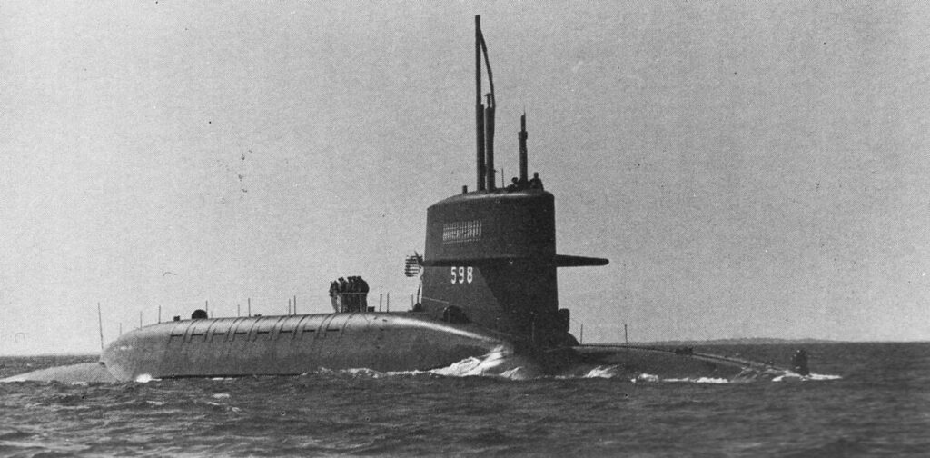
On 15 Nov 1960, the FBM submarine USS George Washington (SSBN-598) embarked on the nation’s first Polaris nuclear deterrent patrol armed with 16 intermediate range Polaris A1 submarine launched ballistic missiles (SLBMs). This milestone occurred just 3 years 11 months after the Polaris FBM program was funded by Congress and authorized by the Secretary of Defense. The 1st deterrent patrol was completed 66 days later on 21 January 1961.
USS George Washington underway. Source: Navsource
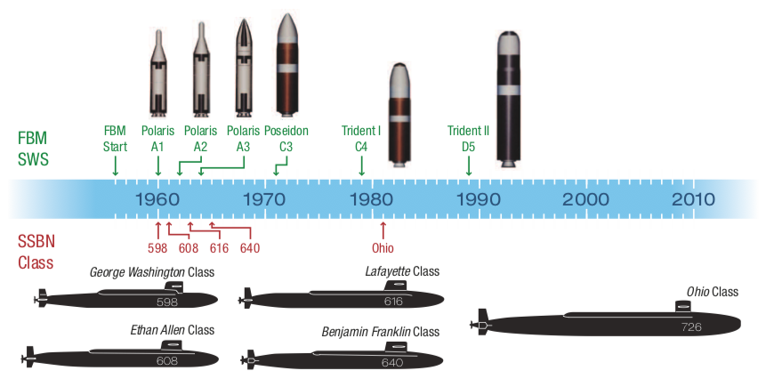
The original US FBM submarine force consisted of 41 Polaris submarines, in five sub-classes (George Washington, Ethan Allen, Lafayette, James Madison and Benjamin Franklin), that were authorized between 1957 and l963. Through several rounds of modifications, most of these submarines were adapted to handle later versions of the Polaris SLBM (A2, A3 and A4) and some were modified to handle the Poseidon (C3) SLBM. Twelve of the James Madison- and Ben Franklin-class boats were modified the late 1970s and early 1980s to handle the long range Trident I C4 SLBMs.
A total of 1,245 Polaris deterrent patrols were made in a period of about 21 years, from the first Polaris A-1 deterrent patrol by USS George Washington in 1960, and ending with the last Polaris A-3 deterrent patrol by USS Robert E. Lee (SSBN-601), which started on 1 October 1981. By then, the remainder of the original Polaris SSBN fleet had transitioned to Poseidon (C3) and Trident I (C4) SLBMs.
The next generation of US ballistic missile submarines was the Ohio-class SSBN, 18 of which were ordered between 1974 and 1990 (one per fiscal year). The lead ship of this class, USS Ohio (SSBN 726), was commissioned in 1981 and deployed 6 September 1982 on its first strategic deterrent patrol, armed with the Trident I (C4) SLBM. Beginning with the 9th boat in class, USS Tennessee (SSBN-734), the remaining Ohio- class SSBNs were equipped originally to handle the larger Trident II (D5). Four of the early boats were upgraded to handle the Trident II (D5) missile. The earliest four, including the USS Ohio, were converted to cruise missile submarines to comply with strategic weapons treaty limits.
Evolution of the US submarine strategic nuclear deterrent fleet. Johns Hopkins APL Technical Digest, Volume 29, Number 4, 2011
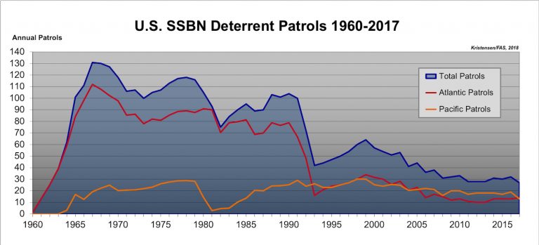
The Federation of American Scientists (FAS) reported that the US Navy conducted 4,086 submarine strategic deterrent patrols between 1969 and 2017. At that time, the Navy was conducting strategic deterrent patrols at a steady rate of around 30 patrols per year. By the end of 2020, that total must be approaching 4,175 patrols.
Source: Hans Kristensen, FAS, 2018
In 2020, the US maintains a fleet of 14 Trident missile submarines armed with D5LE (life extension) SLBMs. By about 2031, the first of the new Columbia-class SSBN is expected to be ready to start its first deterrent patrol. Ohio-class SSBNs will be retired on a one-for-one bases when the new Columbia-class SSBNs are delivered to the fleet and ready to assume deterrent patrol duties.
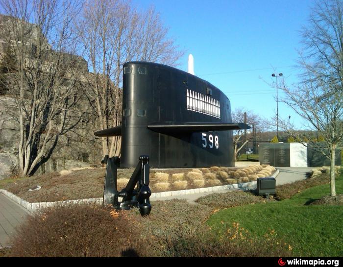
The USS George was defueled and declared scrapped in September 1998. Owing to her place in history as the first US ballistic missile submarine and her successful completion of 55 deterrent patrols in both the Atlantic & Pacific Oceans, the George Washington’s sail was preserved and returned to New London, CT where it is now displayed outside of the gates of the US Submarine Force Library and Museum.
The USS George Washington’s sail on display outside the US Submarine Force Library and Museum in New London, CT. Source: Wikimapia
John Gibson & Stephen Yanek, “The Fleet Ballistic Missile Strategic Weapon System: APL’s Efforts for the U.S. Navy’s Strategic Deterrent System and the Relevance to Systems Engineering,” Johns Hopkins APL Technical Digest, Volume 29, Number 4, 2011: https://www.jhuapl.edu/Content/techdigest/pdf/V29-N04/29-04-Gibsonl.pdf
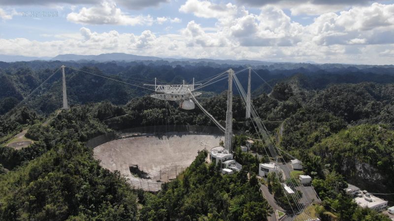
The Arecibo Observatory (AO) on Puerto Rico has been out of service since 10 August 2020, when a three-inch auxiliary support cable slipped out of its socket and fell onto the fragile radio telescope dish below. Three months later, on 6 November 2020, a second cable associated with the same support tower broke, damaging nearby cables, causing more damage to the reflector dish, and leaving the radio telescope’s support structure in a weakened and uncertain state.
On 19 November 2020, the National Science Foundation (NSF) announced it has begun planning for decommissioning the 57-year old Arecibo Observatory’s (AO) 1,000-foot (305-meter) radio telescope due to safety concerns after the two support wires broke and seriously damaged the antenna. You can read NSF News Release 20-010 at the following link: https://www.nsf.gov/news/news_summ.jsp?cntn_id=301674
The 1,000-foot (305-m) dish at Arecibo Observatory in better days, in Spring 2019. Source: AO/University of Central Florida (UCF)The damaged Arecibo Observatory radio telescope in November 2020. Source: NSFA view from under the damaged dish. Source: AO/University of Central Florida (UCF)
Not included in the NSF timeline is the 1974 first-ever broadcast into deep space of a powerful signal that could alert other intelligent life to our technical civilization on Earth. The 1,679 bit “Arecibo Message” was directed toward the globular star cluster M13, which is 22,180 light years away. The message will be in transit for another 22,134 years.
A key capability lost is AO’s planetary radar capability that enabled the large dish to function as a high-resolution, active imaging radar. You’ll find examples of AO’s radar images of the Moon, planets, Jupiter’s satellites, Saturn’s rings, asteroids and comets on the NSF website here: https://www.naic.edu/~pradar/radarpage.html
More impressive than the still images were animations created from a sequence of AO radar images, particularly of passing asteroids. The animations defined the motion of the object as it flew near Earth. As an example, you can watch the following short (1:07 minutes) video, “Big asteroid 1998 OR2 seen in radar imagery ahead of fly-by”:
The US still has a reduced capability for planetary radar imaging with NASA’s Deep-Space Network’s Uplink Array.
The 19 November 2020 NSF news release stated, “After the telescope decommissioning, NSF would intend to restore operations at assets such as the Arecibo Observatory LIDAR facility — a valuable geospace research tool — as well as at the visitor center and offsite Culebra facility, which analyzes cloud cover and precipitation data.”
Adieu to radio astronomy at Arecibo.
Update 1 December 2020: Arecibo radio telescope collapsed.
NPR reported, “The Arecibo Observatory in Puerto Rico has collapsed, after weeks of concern from scientists over the fate of what was once the world’s largest single-dish radio telescope. Arecibo’s 900-ton equipment platform, suspended 500 feet above the dish, fell overnight after the last of its healthy support cables failed to keep it in place. No injuries were reported, according to the National Science Foundation, which oversees the renowned research facility.”
Arecibo after the collapse. Source: Ricardo Arduengo / AFP via Getty Images
Update 8 December 2020: National Science Foundation video shows the moment of collapse.
Update 19 October 2022: No NSF funding
On 18 October 2022, Science magazine reported on NSF’s plans to convert the iconic observatory in Puerto Rico into a center for education and outreach in science, technology, engineering, and math (STEM). The limited funding available for this purpose “does not include support for remaining instruments at the site, including a 12-meter radio telescope, a radio spectrometer, and a suite of optical laser instruments for studying the upper atmosphere.”
The US Geologic Survey (USGS) provides a basic explanation of why glacial ice is blue:
“The red-to-yellow (longer wavelength) parts of the visible spectrum are absorbed by ice more effectively than the blue (shorter wavelength) end of the spectrum. The longer the path light travels in ice, the more blue it appears. This is because the other colors are being preferentially absorbed and make up an ever smaller fraction of the light being transmitted and scattered through the ice.”
Blue ice with natural lighting inside a glacial ice cave, Grindelwald, Switzerland. Source: P. Lobner photo
The key to blue ice is selective absorption, which occurs in a special kind of ice that is produced on land with the help of pressure and time. Becky Oskin provides the following general insights into how this process occurs in her 2015 article, “Why Are Some Glaciers Blue?”
When glacial ice first freezes, it is filled with air bubbles that are effective in scattering light passing through the ice. As that ice gets buried and compressed by subsequent layers of younger ice, the air bubbles become smaller and smaller. With less scattering of light by the air bubbles, light can penetrate more deeply into the ice and the older ice starts to take on a blue tinge. Blue ice is old ice.
Patches of blue-hued ice emerge on the surface of glaciers where wind and sublimation have scoured old glaciers clean of snow and young ice.
Blue ice also may emerge at the edges of a glacial icepack, where fragments of glaciers tumble into the sea and reveal a fresh edge of the old ice.
Stephen Warren’s 2019 paper, “Optical properties of ice and snow,” provides the following more technical description of the selective absorption process in ice:
“Ice is a weak filter for red light..….the absorption coefficient of ice increases with wavelength from blue to red (but the absorption spectrum is quite complex). The absorption length…… is approximately 2 meters at (a wavelength of ) λ = 700 nm (nanometers, red end of the visible spectrum) but approximately 200 meters at λ = 400 nm (blue-violet end of the visible spectrum). Photons at all wavelengths of visible light will survive without absorption, and be reflected or transmitted, unless the path length through ice is long enough to significantly absorb the red light.”…..”Ice develops a noticeable blue color in glacier crevasses and in icebergs, especially in marine ice (i.e., icebergs calved from glacial ice shelves), because of its lack of (air) bubbles (which would otherwise cause scattering and limit light transmission through the ice).”
The absorption length is the distance into a material where the beam flux has dropped to 1/e (1/2.71828 = 0.368 = 37%) of its incident flux. For light at the red end of the spectrum, that is a relatively short distance of about 2 meters. This means that, in 2 meters, absorption decreases the red light component of beam flux by a factor of 1/e to about 37% of the original incident red light. In another 2 meters, the red light beam flux is reduced to about 14% of the original incident red light. At the same distances, the blue-violet end of the spectrum has hardly been attenuated at all.
You can see that even modest size pieces of glacial ice (several meters in length / diameter) should be able to attenuate the red-to-yellow end of the spectrum and appear with varying degrees of blue tints. Looking into an ice borehole in an Antarctic ice sheet shows how intensely blue the deeper part of the glacial ice appears to the viewer on the surface. The removed ice core is a slender cylinder of ice that looks like clear ice when viewed from the side.
So… why is snow white? Light does not penetrate into snow very far before being scattered back to the viewer by the many facets of uncompressed snow on the surface. Thus, there is almost no opportunity for light absorption by the snow, and hence very little selective absorption of the red-to-yellow part of the visible spectrum.
For the same reason, sea ice, which is formed by the seasonal freezing of the sea surface, appears white because of the high concentration of entrained air bubbles (relative to glacial ice) that causes rapid scattering of incident light. Sea ice does not go through the metamorphism that produces glacial ice on land.
What is glacial ice?
The USGS describes glacial ice as follows: “Glacier ice is actually a mono-mineralic rock (a rock made of only one mineral, like limestone which is composed of the mineral calcite). The mineral ice is the crystalline form of water (H2O). It forms through the metamorphism of tens of thousands of individual snowflakes into crystals of glacier ice. Each snowflake is a single, six-sided (hexagonal) crystal with a central core and six projecting arms. The metamorphism process is driven by the weight of overlying snow. During metamorphism, hundreds, if not thousands of individual snowflakes recrystallize into much larger and denser individual ice crystals. Some of the largest ice crystals observed at Alaska’s Mendenhall Glacier are nearly one foot in length.”
A small chunk of clear glacial ice retrieved from Pléneau Bay, Antarctica. Source: P. Lobner photo
Where do glaciers exist?
The National Snow and Ice Data Center (NSIDC) reports that, “glaciers occupy about 10 percent of the world’s total land area, with most located in polar regions like Antarctica, Greenland, and the Canadian Arctic. Glaciers can be thought of as remnants from the last Ice Age, when ice covered nearly 32 percent of the land, and 30 percent of the oceans. Most glaciers lie within mountain ranges that show evidence of a much greater extent during the ice ages of the past two million years, and more recent indications of retreat in the past few centuries.”
Glaciers exist on every continent except Australia. The approximate distribution of glaciers is:
91% in Antarctica
8% in Greenland
Less than 0.5% in North America (about 0.1% in Alaska)
0.2% in Asia
Less than 0.1% is in South America, Europe, Africa, New Zealand, and New Guinea (Irian Jaya).
There are several schemes for classifying glaciers; some are described in the references at the end of this article. For simplicity, let’s consider two basic types.
A polar glacier is defined as one that is below the freezing temperature throughout its mass for the entire year. Polar glaciers exist in Antarctica and Greenland as continental scale ice sheets and smaller scale ice caps and ice fields.
A temperate glacier is a glacier that’s essentially at the melting point, so liquid water coexists with glacier ice. A small change in temperature can have a major impact on temperate glacier melting, area, and volume. Glaciers not in Antarctica or Greenland are temperate glaciers. In addition, some of the glaciers on the Antarctic Peninsula and some of Greenland’s southern outlet glaciers are temperate glaciers.
How old is glacier ice?
Some glacial ice is extremely old, while in many areas of the world, it is much younger than you might have expected.
USGS reports: “Parts of the Antarctic Continent have had continuous glacier cover for perhaps as long as 20 million years. Other areas, such as valley glaciers of the Antarctic Peninsula and glaciers of the Transantarctic Mountains may date from the early Pleistocene (starting about 2.6 million years ago and lasting until about 11,700 years ago). For Greenland, ice cores and related data suggest that all of southern Greenland and most of northern Greenland were ice-free during the last interglacial period, approximately 125,000 years ago. Then, climate (in Greenland) was as much as 3-5o F warmer than the interglacial period we currently live in.”
“Although the higher mountains of Alaska have hosted glaciers for as much as the past 4 million years, most of Alaska temperate glaciers are generally much, much younger. Many formed as recently as the start of the Little Ice Age, approximately 1,000 years ago. Others may date from other post-Pleistocene (younger than 11,700 years ago) colder climate events.”
The age of the oldest glacier ice in Antarctica may approach 20,000,000 years old.
The age of the oldest glacier ice in Greenland may be more than 100,000 years old, but less than 125,000 years old.
The age of the oldest Alaskan glacier ice ever recovered was about 30,000 years old.
Blue glacial ice along the coast of the West Antarctic Peninsula
In February 2020, my wife and I made a well-timed visit to the West Antarctic Peninsula. One particularly amazing spot was Pléneau Bay, which easily could earn the title “Antarctic Museum of Modern Art” because of the many fanciful iceberg shapes floating gently in this quiet bay. Following is a short photo essay highlighting several of the beautiful blue glacial ice features we saw on this trip.
Small blue iceberg in the Lemaire Channel. Source: P. Lobner photoZodiacs in what could be called the “Antarctic Museum of Modern Art” in Pléneau Bay. Source: J. Lobner photoCrabeater seal amid the blue icebergs in Pléneau Bay. Source: J. Lobner photoExotic blue iceberg shapes in Pléneau Bay. Source: P. Lobner photoThe tall, fluted wall of a large blue iceberg in Pléneau Bay. Source: J. Lobner photoA chunk of faceted glacial ice among the brash sea ice in Hanusse Bay / Crystal Sound. Source: P. Lobner photoBlue icebergs among the brash sea ice at Prospect Point (above & below). Source: P. Lobner photosA humpback whale resting among the blue icebergs in Cierva Cove (above) and diving (below). Source: P. Lobner photosThis iceberg (above & below) in Cierva Cove looks like a majestic blue sailing ship. Source: P. Lobner photosAnother exotic blue iceberg in Cierva Cove. Source: J. Lobner photoZodiac among blue icebergs in Cierva Cove. Source: P. Lobner photoThe large underwater part of this iceberg radiates blue in Cierva Cove. Source: P. Lobner photoA sea cave provides a view into the blue ice underlying an ice shelf. Source: P. Lobner photo
Examples of blue glacial ice in Switzerland & New Zealand
In previous years, my wife and I visited a temperate glacier and ice cave in Grindelwald, Switzerland and hiked on the temperate Franz Josef Glacier on the South Island of New Zealand. Following is a short photo essay that should give you an idea of the complex terrain of these glaciers and the smaller scale blue ice features visible on the surface. In contrast, the ice cave was a unique, immersive, very blue experience. The blue color inside the cave looked like the eerie blue light from Cherenkov radiation, like you’d see in an operating pool-type nuclear research reactor.
Inside a glacial ice cave in Grindelwald, Switzerland. Source: P. Lobner photoFranz Joseph Glacier showing a general blue tint in some surface ice (above) and more intense blue in smaller areas (below), South Island, New Zealand. Source: P. Lobner photosFranz Joseph Glacier details (above & below). Source: P. Lobner photos
Festo is a German multinational industrial control and automation company based in Esslingen am Neckar, near Stuttgart. The Festo website is here: https://www.festo.com/group/en/cms/10054.htm
Festo reports that they invest about 8% of their revenues in research and development. Festo’s draws inspiration for some of its control and automation technology products from the natural world. To help facilitate this, Festo established the Bionic Learning Network, which is a research network linking Festo to universities, institutes, development companies and private inventors. A key goal of this network is to learn from nature and develop “new insights for technology and industrial applications”…. “in various fields, from safe automation and intelligent mechatronic solutions up to new drive and handling technologies, energy efficiency and lightweight construction.”
One of the challenges taken on by the Bionic Learning Network was to decipher how birds fly and then develop robotic devices that can implement that knowledge and fly like a bird. Their first product was the 2011 SmartBird and their newest product is the 2020 BionicSwift. In this article we’ll take a look at these two bionic birds and the significant advancements that Festo has made in just nine years.
2. SmartBird
On 24 March 2011, Festo issued a press release introducing their SmartBird flying bionic robot, which was one of their 2011 Bionic Learning Network projects. Festo reported:
“The research team from the family enterprise Festo has now, in 2011, succeeded in unraveling the mystery of bird flight. The key to its understanding is a unique movement that distinguishes SmartBird from all previous mechanical flapping wing constructions and allows the ultra-lightweight, powerful flight model to take off, fly and land autonomously.”
“SmartBird flies, glides and sails through the air just like its natural model – the Herring Gull – with no additional drive mechanism. Its wings not only beat up and down, but also twist at specific angles. This is made possible by an active articulated torsional drive unit, which in combination with a complex control system makes for unprecedented efficiency in flight operation. Festo has thus succeeded for the first time in attaining an energy-efficient technical adaptation of this model from nature.”
SmartBird measures 1.07 meters (42 in) long with a wingspan of 2.0 meters (79 in) and a weigh of 450 grams (16 ounces, 1 pound). This is about a 1.6X scale-up in the length and span of an actual Herring Gull, but at about one-third the weight. It is capable of autonomous takeoff, flight, and landing using just its wings, and it controls itself the same way birds do, by twisting its body, wings, and tail. SmartBird’s propulsion system has a power requirement of 23 watts.
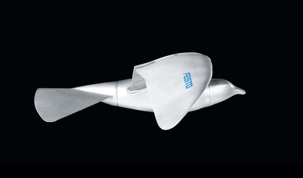
On 1 July 2020, Festo introduced the BionicSwift as their latest ultra light flying bionic robot that mimics how actual birds fly.
The BionicSwift, inspired by a Common Swift, measures 44.5 cm (17.5 in) long with a wingspan of 68 cm (26.7 in) and a weight of just 42 grams (1.5 ounces). It’s approximately a 2X scale-up of a Common Swift, but still a remarkably compact, yet complex flying machine with aerodynamic plumage that closely replicates the flight feathers on an actual Swift. The 2011 SmartBird was more than twice the physical size and ten times heavier.
The BionicSwift is agile, nimble and can even fly loops and tight turns. Festo reports: “Due to this close-to-nature replica of the wings, the BionicSwifts have a better flight profile than previous wing-beating drives.” Compare the complex, feathered wing structure in the following Festo photos of the BionicSwift with the previous photos showing the simpler, solid wing structure of the 2011 SmartBird.
Source: All three BionicSwift photos from Festo
A BionicSwift can fly singly or in coordinated flight with a group of other BionicSwifts. Festo describes how this works: “Radio-based indoor GPS with ultra wideband technology (UWB) enables the coordinated and safe flying of the BionicSwifts. For this purpose, several radio modules are installed in one room. These anchors then locate each other and define the controlled airspace. Each robotic bird is also equipped with a radio marker. This sends signals to the anchors, which can then locate the exact position of the bird and send the collected data to a central master computer, which acts as a navigation system.” Flying time is about seven minutes per battery charge.
4. For more information about other Festo bionic creations:
I encourage you to visit the Festo BionIc Learning Network webpage at the following link and browse the resources available for the many intriguing projects. https://www.festo.com/group/en/cms/10156.htm
On this webpage you’ll find a series of links listed under the heading “More Projects,” which will introduce you to the wide range of Bionic Learning Network projects since 2006.
You also can watch the following YouTube short videos of Festo’s many bionic creations:
BionicFinWave (2018):replicates the swimming movements of sea creatures with undulating fins to create a unique fin drive system for an autonomous underwater vehicle: https://www.youtube.com/watch?v=fRNq55EbnZc
AirRay (2010): replicates the natural underwater movements of a Manta Ray in a larger-than-life, neutrally buoyant, ray-shaped airship with a flapping wing drive: https://www.youtube.com/watch?v=c3-wIICjAhE
AquaRay (2010): replicates the natural underwater movements of a Manta Ray in a full-size autonomous underwater vehicle with a flapping wing drive: https://www.youtube.com/watch?v=F4-6oNagIvk
AirPenguin (2009): replicates the natural underwater movements of a penguin in a larger-than-life, neutrally buoyant, penguin-shaped airship: https://www.youtube.com/watch?v=jPGgl5VH5go
AquaPenguin (2009): replicates the natural underwater movements of a penguin in a small penguin-sized autonomous underwater vehicle: https://www.youtube.com/watch?v=u8tfES8gImc
AirJelly (2008): replicates the natural underwater movements of a jelly fish in a larger-than-life, neutrally buoyant, jelly fish-shaped airship: https://www.youtube.com/watch?v=divLsTtA5vk
AquaJelly (2008): replicates the natural underwater movements of a jelly fish in a small, autonomous, peristaltic drive autonomous underwater vehicle that can operate in coordination with several other AquaJellies: https://www.youtube.com/watch?v=N-O8-N71Qcw
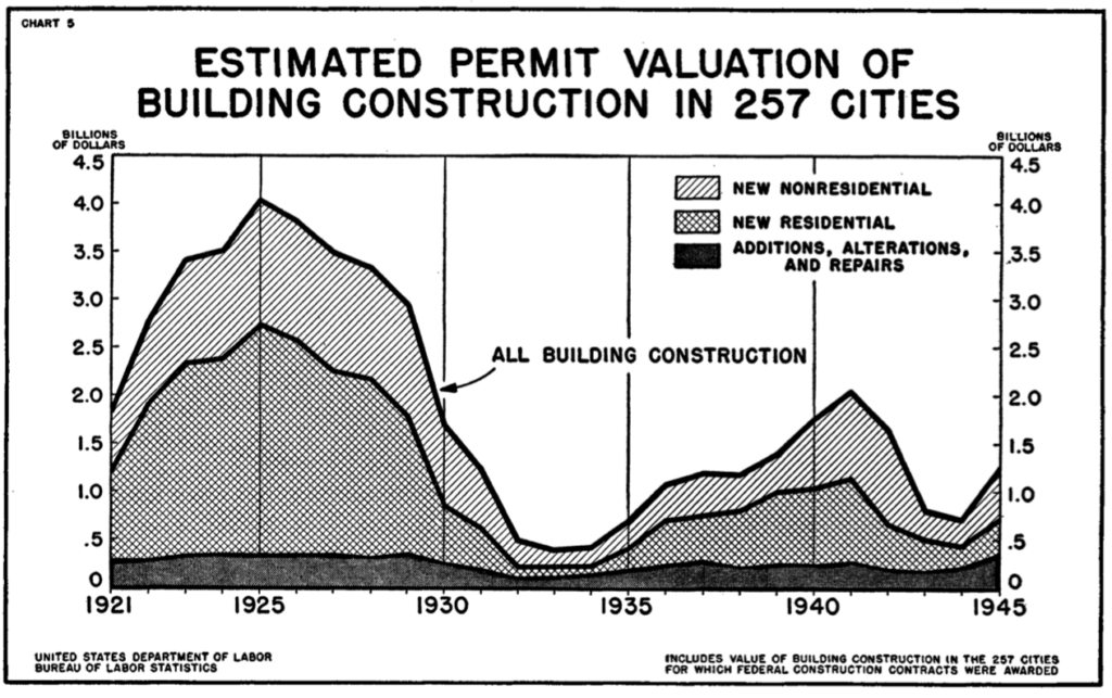
At the start of World War II (WW II), US home ownership had dropped to a low of 43.6% in 1940, largely as a consequence of the Great Depression and the weak US economy in its aftermath. During WW II, the War Production Board issued Conservation Order L-41 on 9 April 1942, placing all construction under rigid control. The order made it necessary for builders to obtain authorization from the War Production Board to begin construction costing more than certain thresholds during any continuous 12-month period. For residential construction, that limit was $500, with higher limits for business and agricultural construction. The impact of these factors on US residential construction between 1921 and 1945 is evident in the following chart, which shows the steep decline during the Great Depression and again after Order L-41 was issued.
Source: “Construction in the War Years – 1942 -45,” US Department of Labor, Bulletin No. 915
By the end of WW II, the US had an estimated 7.6 million troops overseas. The War Production Board revoked L-41 on 15 October 1945, five months after V-E (Victory in Europe) day on 8 May 1945 and six weeks after WW II ended when Japan formally surrendered on 2 September 1945. In the five months since V-E day, about three million soldiers had already returned to the US. After the war’s end, the US was faced with the impending return of several millions more veterans. Many in this huge group of veterans would be seeking to buy homes in housing markets that were not prepared for their arrival. Within the short span of a year after Order L-41 was revoked, the monthly volume of private housing expenditures increased fivefold. This was just the start of the post-war housing boom in the US.
In a March 1946 Popular Science magazine article entitled “Stopgap Housing,” the author, Hartley Howe, noted, “ Even if 1,200,000 permanent homes are now built every year – and the United States has never built even 1,000,000 in a single year – it will be 10 years before the whole nation is properly housed. Hence, temporary housing is imperative to stop that gap.” To provide some immediate relief, the Federal government made available many thousands of war surplus steel Quonset huts for temporary civilian housing.
Facing a different challenge in the immediate post-war period, many wartime industries had their contracts cut or cancelled and factory production idled. With the decline of military production, the U.S. aircraft industry sought other opportunities for employing their aluminum, steel and plastics fabrication experience in the post-war economy.
2. Post-WW II prefab aluminum and steel houses in the US
In the 2 September 1946 issue of Aviation News magazine, there was an article entitled “Aircraft Industry Will Make Aluminum Houses for Veterans,” that reported the following:
“Two and a half dozen aircraft manufacturers are expected soon to participate in the government’s prefabricated housing program.”
“Aircraft companies will concentrate on FHA (Federal Housing Administration) approved designs in aluminum and its combination with plywood and insulation, while other companies will build prefabs in steel and other materials. Designs will be furnished to the manufacturers.”
“Nearly all war-surplus aluminum sheet has been used up for roofing and siding in urgent building projects; practically none remains for the prefab program. Civilian Production Administration has received from FHA specifications for aluminum sheet and other materials to be manufactured, presumably under priorities. Most aluminum sheet for prefabs will be 12 to 20 gauge – .019 – .051 inch.”
In October 1946, Aviation News magazine reported, “The threatened battle over aluminum for housing, for airplanes and myriad postwar products in 1947 is not taken too seriously by the National Housing Agency, which is negotiating with aircraft companies to build prefabricated aluminum panel homes at an annual rate as high as 500,000.”……”Final approval by NHA engineers of the Lincoln Homes Corp. ‘waffle’ panel (aluminum skins over a honeycomb composite core) is one more step toward the decision by aircraft companies to enter the field.…..Aircraft company output of houses in 1947, if they come near meeting NHA proposals, would be greater than their production of airplanes, now estimated to be less than $1 billion for 1946.”
In late 1946, the FHA Administrator, Wilson Wyatt, suggested that the War Assets Administration (WAA), which was created in January 1946 to dispose of surplus government-owned property and materials, temporarily withhold surplus aircraft factories from lease or sale and give aircraft manufacturers preferred access to surplus wartime factories that could be converted for mass-production of houses. The WAA agreed.
Under the government program, the prefab house manufacturers would have been protected financially with FHA guarantees to cover 90% of costs, including a promise by Reconstruction Finance Corporation (RFC) to purchase any homes not sold.
Many aircraft manufacturers held initial discussions with the FHA, including: Douglas, McDonnell, Martin, Bell, Fairchild, Curtis-Wright, Consolidated-Vultee, North American, Goodyear and Ryan. Boeing did not enter those discussions and Douglas, McDonnell and Ryan exited early. In the end, most aircraft manufacturer were unwilling to commit themselves to the postwar prefab housing program, largely because of their concerns about disrupting their existing aircraft factory infrastructure based on uncertain market estimates of size and duration of the prefab housing market and lack of specific contract proposals from the FHA and NHA.
The original business case for the post-war aluminum and steel pre-fabricated houses was that they could be manufactured rapidly in large quantities and sold profitably at a price that was less than conventional wood-constructed homes. Moreover, the aircraft manufacturing companies restored some of the work volume lost after WW II ended and they were protected against the majority of their financial risk in prefab house manufacturing ventures.
Not surprisingly, building contractors and construction industry unions were against this program to mass-produce prefabricated homes in factories, since this would take business away from the construction industry. In many cities the unions would not allow their members to install prefabricated materials. Further complicating matters, local building codes and zoning ordnances were not necessarily compatible with the planned large-scale deployment of mass-produced, prefabricated homes.
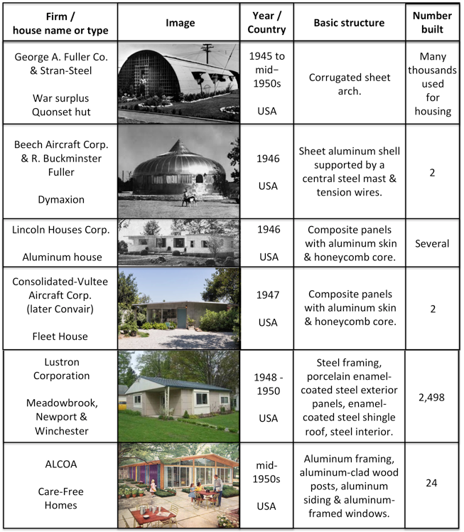
The optimistic prospects for manufacturing and erecting large numbers of prefabricated aluminum and steel homes in post-WW II USA never materialized. Rather than manufacturing hundreds of thousands of homes per year, the following five US manufacturers produced a total of less than 2,600 new aluminum and steel prefabricated houses in the decade following WW II: Beech Aircraft, Lincoln Houses Corp., Consolidated-Vultee, Lustron Corp. and Aluminum Company of America (Alcoa). In contrast, prefabricators offering more conventional houses produced a total of 37,200 units in 1946 and 37,400 in 1947. The market demand was there, but not for aluminum and steel prefabricated houses.
US post-WW II prefabricated aluminum and steel houses
These US manufacturers didn’t play a significant part in helping to solve the post-WW II housing shortage. Nonetheless, these aluminum and steel houses still stand as important examples of affordable houses that, under more favorable circumstances, could be mass-produced even today to help solve the chronic shortages of affordable housing in many urban and suburban areas in the US.
Some of the US post-WW II housing demand was met with stop gap, temporary housing using re-purposed, surplus wartime steel Quonset huts, military barracks, light-frame temporary family dwelling units, portable shelter units, trailers, and “demountable houses,” which were designed to be disassembled, moved and reassembled wherever needed. You can read more about post-WW II stop gap housing in the US in Hartley Howe’s March 1946 article in Popular Science (see link below).
The construction industry ramped up rapidly after WW II to help meet the housing demand with conventionally-constructed permanent houses, with many being built in large-scale housing tracts in rapidly expanding suburban areas. Between 1945 and 1952, the Veterans Administration reported that it had backed nearly 24 million home loans for WW II veterans. These veterans helped boost US home ownership from 43.6% in 1940 to 62% in 1960.
Two post-WW II US prefabricated aluminum and steel houses have been restored and are on public display in the following museums:
In addition, you can visit several WW II Quonset huts at the Seabees Museum and Memorial Park in North Kingstown, Rhode Island. None are outfitted like a post-WW II civilian apartment. The museum website is here: https://www.seabeesmuseum.com
You’ll find more information in my articles on specific US post-WW II prefabricated aluminum and steel houses at the following links:
3. Post-WW II prefab aluminum and steel houses in the UK
By the end of WW II in Europe (V-E Day is 8 May 1945), the UK faced a severe housing shortage as their military forces returned home to a country that had lost about 450,000 homes to wartime damage.
On 26 March 1944, Winston Churchill made an important speech promising that the UK would manufacture 500,000 prefabricated homes to address the impending housing shortage. Later in the year, the Parliament passed the Housing (Temporary Accommodation) Act, 1944, charging the Ministry of Reconstruction with developing solutions for the impending housing shortage and delivering 300,000 units within 10 years, with a budget of £150 million.
The Act provided several strategies, including the construction of temporary, prefabricated housing with a planned life of up to 10 years. The Temporary Housing Program (THP) was officially known as the Emergency Factory Made (EFM) housing program. Common standards developed by the Ministry of Works (MoW) required that all EFM prefabricated units have certain characteristics, including:
Minimum floor space of 635 square feet (59 m2)
Maximum width of prefabricated modules of 7.5 feet (2.3 m) to enable transportation by road throughout the country
Implement the MoW’s concept of a “service unit,” which placed the kitchen and bathroom back-to-back to simplify routing plumbing and electrical lines and to facilitate factory manufacture of the unit.
Factory painted, with “magnolia” (yellow-white) as the primary color and gloss green as the trim color.
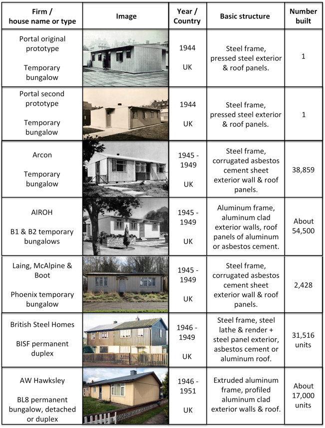
In 1944, the UK Ministry of Works held a public display at the Tate Gallery in London of five types of prefabricated temporary houses.
The original Portal all-steel prototype bungalow
The AIROH (Aircraft Industries Research Organization on Housing) aluminum bungalow, made from surplus aircraft material.
The Arcon steel-framed bungalow with asbestos concrete panels. This deign was adapted from the all-steel Portal prototype.
Two timber-framed prefab designs, the Tarran and the Uni-Seco
This popular display was held again in 1945 in London.
Supply chain issues slowed the start of the EFM program. The all-steel Portal was abandoned in August 1945 due to a steel shortage. In mid-1946, a wood shortage affected other prefab manufacturers. Both the AIROH and Arcon prefab houses were faced with unexpected manufacturing and construction cost increases, making these temporary bungalows more expensive to build than conventionally constructed wood and brick houses.
Under a Lend-Lease Program announced in February 1945, the US agreed to supply the UK with US-built, wood frame prefabricated bungalows known as the UK 100. The initial offer was for 30,000 units, which subsequently was reduced to 8,000. This Lend-Lease agreement came to an end in August 1945 as the UK started to ramp up its own production of prefabricated houses. The first US-built UK 100 prefabs arrived in late May/early June 1945.
The UK’s post-war housing reconstruction program was quite successful, delivering about 1.2 million new houses between 1945 and 1951. During this reconstruction period, 156,623 temporary prefabricated homes of all types were delivered under the EFM program, which ended in 1949, providing housing for about a half million people. Over 92,800 of these were temporary aluminum and steel bungalows. The AIROH aluminum bungalow was the most popular EFM model, followed by the Arcon steel frame bungalow and then the wood frame Uni-Seco. In addition, more than 48,000 permanent aluminum and steel prefabricated houses were built by AW Hawksley and BISF during that period.
In comparison to the very small number of post-war aluminum and steel prefabricated houses built in the US, the post-war production of aluminum and steel prefabs in the UK was very successful.
UK post-WW II prefabricated aluminum and steel houses
In a 25 June 2018 article in the Manchester Evening News, author Chris Osuh reported that, “It’s thought that between 6 or 7,000 of the post-war prefabs remain in the UK…..” The Prefab Museum maintains a consolidated interactive map of known post-WW II prefab house locations in the UK at the following link: https://www.prefabmuseum.uk/content/history/map
Screenshot of the Prefab Museum’s interactive map (not including the prefabs in the Shetlands, which are off the top of this screenshot).
In the UK, Grade II status means that a structure is nationally important and of special interest. Only a few post-war temporary prefabs have been granted the status as Grade II listed properties:
In an estate of Phoenix steel frame bungalows built in 1945 on Wake Green Road, Moseley, Birmingham, 16 of 17 homes were granted Grade II status in 1998.
Six Uni-Seco wood frame bungalows built in 1945 – 46 in the Excalibur Estate, Lewisham, London were granted Grade II status in 2009. At that time, Excalibur Estates had the largest number of WW II prefabs in the UK: 187 total, of several types.
Several post-war temporary prefabs are preserved at museums in the UK and are available to visit.
St. Fagans National Museum of History in Cardiff, South Wales: An AIROH B2 originally built near Cardiff in 1947 was dismantled and moved to its current museum site in 1998 and opened to the public in 2001. You can see this AIROH B2 here: https://museum.wales/stfagans/buildings/prefab/
Chiltern Open Air Museum (COAM) in Chalfont St. Giles, Buckinghamshire: Their collection includes a wood frame Universal House Mark 3 prefab manufactured by Universal Housing Company of Rickmansworth, Hertfordshire. This prefab was built in 1947 in the Finch Lane Estate in Amersham. You can see the “Amersham Prefab” here: https://www.coam.org.uk/museum-buckinghamshire/historic-buildings/amersham-prefab/
I think the Prefab Museum is best source for information on UK post-WW II prefabs. When it was created in March 2014 by Elisabeth Blanchet (author of several books and articles on UK prefabs) and Jane Hearn, the Prefab Museum had its home in a vacant prefab on the Excalibur Estate in south London. After a fire in October 2014, the physical museum closed but has continued its mission to collect and record memories, photographs and memorabilia, which are presented online via the Prefab Museum’s website at the following link: https://www.prefabmuseum.uk
You’ll find more information in my articles on specific UK post-WW II prefabricated aluminum and steel houses at the following links:
4. Post-WW II prefab aluminum and steel houses in France
At the end of WW II, France, like the UK, had a severe housing shortage due to the great number of houses and apartments damaged or destroyed during the war years, the lack of new construction during that period, and material shortages to support new construction after the war.
To help relieve some of the housing shortage in 1945, the French Reconstruction and Urbanism Minister, Jean Monnet, purchased the 8,000 UK 100 prefabricated houses that the UK had acquired from the US under a Lend-Lease agreement. These were erected in the Hauts de France (near Belgium), Normandy and Brittany, where many are still in use today.
The Ministry of Reconstruction and Town Planning established requirements for temporary housing for people displaced by the war. Among the initial solutions sought were prefabricated dwellings measuring 6 x 6 meters (19.6 x 19.6 feet); later enlarged to 6 × 9 meters (19.6 x 29.5 feet).
About 154,000 temporary houses (the French called then “baraques”), in many different designs, were erected in France in the post-war years, primarily in the north-west of France from Dunkirk to Saint-Nazaire. Many were imported from Sweden, Finland, Switzerland, Austria and Canada.
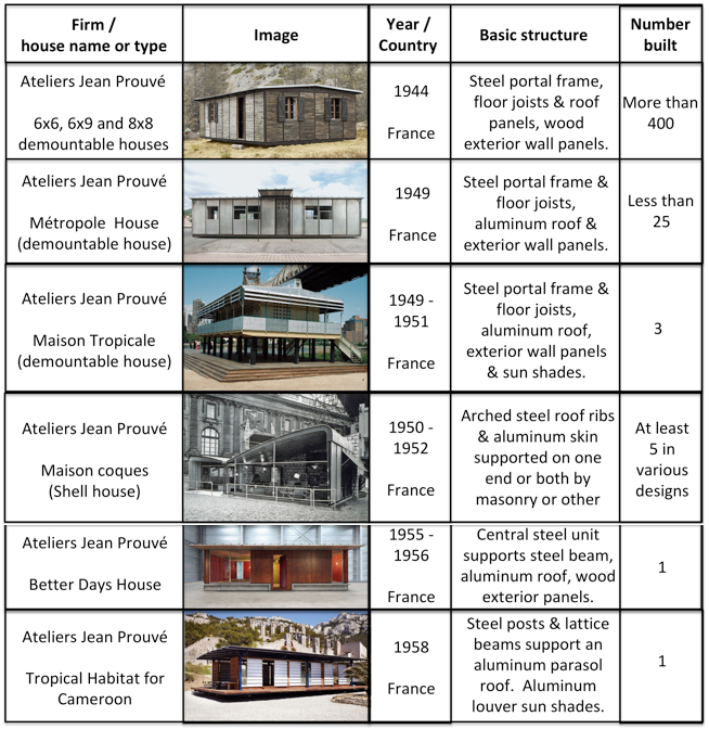
The primary proponent of French domestic prefabricated aluminum and steel house manufacturing was Jean Prouvé, who offered a novel solution for a “demountable house,” which could be easily erected and later “demounted” and moved elsewhere if needed. A steel gantry-like “portal frame” was the load-bearing structure of the house, with the roof usually made of aluminum, and the exterior panels made of wood, aluminum or composite material. Many of these were manufactured in the size ranges requested by Ministry of Reconstruction. During a visit to Prouvé’s Maxéville workshop in 1949, Eugène Claudius-Petit, then the Minister of Reconstruction and Urbanism, expressed his determination to encourage the industrial production of “newly conceived (prefabricated) economical housing.”
French post-WW II prefabricated aluminum and steel houses
Today, many of Prouvé’s demountable aluminum and steel houses are preserved by architecture and art collectors Patrick Seguin (Galerie Patrick Seguin) and Éric Touchaleaume (Galerie 54 and la Friche l’Escalette). Ten of Prouvé’s Standard Houses and four of his Maison coques-style houses built between 1949 – 1952 are residences in the small development known as Cité “Sans souci,” in the Paris suburbs of Muedon.
Prouvé’s 1954 personal residence and his relocated 1946 workshop are open to visitors from the first weekend in June to the last weekend in September in Nancy, France. The Musée des Beaux-Arts de Nancy has one of the largest public collections of objects made by Prouvé.
Author Elisabeth Blanchet reports that the museum “Mémoire de Soye has managed to rebuild three different ‘baraques’: a UK 100, a French one and a Canadian one. They are refurbished with furniture from the war and immediate post-war era. Mémoire de Soye is the only museum in France where you can visit post-war prefabs.” The museum is located in Lorient, Brittany. Their website (in French) is here: http://www.soye.org
The three wood frame ‘baraques’ at Mémoire de Soye. Source: Elisabeth Blanchet via the Prefab Museum (UK)
In the U.S., the post-war mass production of prefabricated aluminum and steel houses never materialized. Lustron was the largest manufacturer with 2,498 houses. In the UK, over 92,800 prefabricated aluminum and steel temporary bungalows were built as part of the post-war building boom that delivered a total of 156,623 prefabricated temporary houses of all types between 1945 and 1949, when the program ended. In France, hundreds of prefabricated aluminum and steel houses were built after WW II, with many being used initially as temporary housing for people displaced by the war. Opportunities for mass production of such houses did not develop in France.
The lack of success in the U.S. arose from several factors, including:
High up-front cost to establish a mass-production line for prefabricated housing, even in a big, surplus wartime factory that was available to the house manufacturer on good financial terms.
Immature supply chain to support a house manufacturing factory (i.e., different suppliers are needed than for the former aircraft factory).
Ineffective sales, distribution and delivery infrastructure for the manufactured houses.
Diverse, unprepared local building codes and zoning ordnances stood in the way of siting and erecting standard design, non-conventional prefab homes.
Opposition from construction unions and workers that did not want to lose work to factory-produced homes.
Only one manufacturer, Lustron, produced prefab houses in significant numbers and potentially benefitted from the economics of mass production. The other manufacturers produced in such small quantities that they could not make the transition from artisanal production to mass production.
Manufacturing cost increases reduced or eliminated the initial price advantage predicted for the prefabricated aluminum and steel houses, even for Lustron. They could not compete on price with comparable conventionally constructed houses.
In Lustron’s case, charges of corporate corruption led the Reconstruction Finance Corporation to foreclose on Lustron’s loans, forcing the firm into an early bankruptcy.
From these post-WW II lessons learned, and with the renewed interest in “tiny homes”, it seems that there should be a business case for a modern, scalable, smart factory for the low-cost mass-production of durable prefabricated houses manufactured from aluminum, steel, and/or other materials. These prefabricated houses could be modestly-sized, modern, attractive, energy efficient (LEED-certified), and customizable to a degree while respecting a basic standard design. These houses should be designed for mass production and siting on small lots in urban and suburban areas. I believe that there is a large market in the U.S. for this type of low-price housing, particularly as a means to address the chronic affordable housing shortages in many urban and suburban areas. However, there still are great obstacles to be overcome, especially where construction industry labor unions are likely to stand in the way and, in California, where nobody will want a modest prefabricated house sited next to their McMansion.
You can download a pdf copy of this post, not including the individual articles, here:
Blaine Stubblefield, “Aircraft Industry Will Make Aluminum Houses for Veterans,” Aviation News, Vol. 6, No. 10, 2 September 1946 (available in the Aviation Week & Space Technology magazine online archive)
“Battle for Aluminum Discounted by NHA,” Aviation News magazine, p. 22, 14 October 1946 (available in the Aviation Week & Space Technology magazine online archive)
Nicole C. Rudolph, “At Home in Postwar France – Modern Mass Housing and the Right to Comfort,” Berghahn Monographs in French Studies (Book 14), Berghahn Books, March 2015, ISBN-13: 978-1782385875. The introduction to this book is available online at the following link: https://berghahnbooks.com/downloads/intros/RudolphAt_intro.pdf
Kenny Cupers, “The Social Project: Housing Postwar France,” University Of Minnesota Press, May 2014, ISBN-13: 978-0816689651
On 20 April 2020, the U.S. Geological Survey (USGS) released the first-ever comprehensive digital geologic map of the Moon. The USGS described this high-resolution map as follows:
“The lunar map, called the ‘Unified Geologic Map of the Moon,’ will serve as the definitive blueprint of the moon’s surface geology for future human missions and will be invaluable for the international scientific community, educators and the public-at-large.”
Color-coded orthographic projections of the “Unified Geologic Map of the Moon” showing the geology of the Moon’s near side (left) and far side (right). Source: NASA/GSFC/USGS
This remarkable mapping product is the culmination of a decades-long project that started with the synthesis of six Apollo-era (late 1960s – 1970s) regional geologic maps that had been individually digitized and released in 2013 but not integrated into a single, consistent lunar map.
This intermediate mapping product was updated based on data from the following more recent lunar satellite missions:
The Lunar Reconnaissance Orbiter Camera (LROC) is a system of three cameras that capture high resolution black and white images and moderate resolution multi-spectral images of the lunar surface: http://lroc.sese.asu.edu
Topography for the north and south poles was supplemented with Lunar Orbiter Laser Altimeter (LOLA) data: https://lola.gsfc.nasa.gov
The final product is a seamless, globally consistent map that is available in several formats: geographic information system (GIS) format at 1:5,000,000-scale, PDF format at 1:10,000,000-scale, and jpeg format.
At the following link, you can download a large zip file (310 Mb) that contains a jpeg file (>24 Mb) with a Mercator projection of the lunar surface between 57°N and 57°S latitude, two polar stereographic projections of the polar regions from 55°N and 55°S latitudes to the poles, and a description of the symbols and color coding used in the maps.
These high-resolution maps are great for exploring the lunar surface in detail. A low-resolution copy (not suitable for browsing) is reproduced below.
For more information on the Unified Geologic Map of the Moon, refer to the paper by C. M. Fortezzo, et al., “Release of the digital Unified Global Geologic Map of the Moon at 1:5,000,000-scale,” which is available here: https://www.hou.usra.edu/meetings/lpsc2020/pdf/2760.pdf
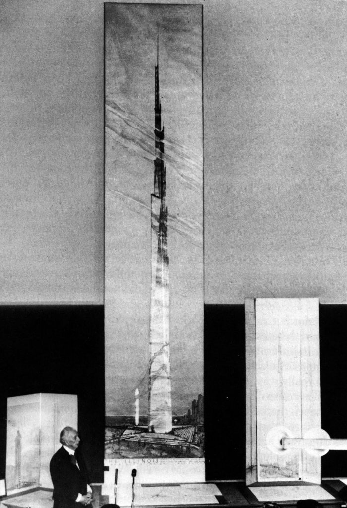
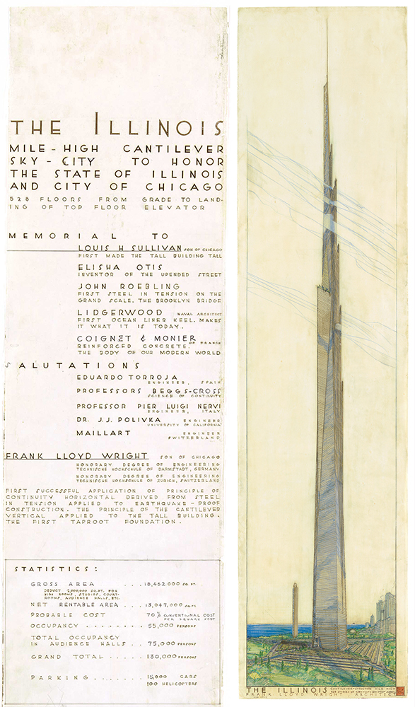
On 16 October 1956, architect Frank Lloyd Wright, then 89 years old, unveiled his design for the tallest skyscraper in the world, a remarkable mile-high tripod spire named “The Illinois,” proposed for a site in Chicago.
Frank Lloyd Wright. Source: Al Ravenna via Wikipedia
Also known as the Illinois Mile-High Tower, Wright’s skyscraper would stand 528 floors and 5,280 feet (1,609 meters) tall plus antenna; more than four times the height of the Empire State Building in New York City, then the tallest skyscraper in the world at 102 floors and 1,250 feet (380 meters) tall plus antenna. At the unveiling of The Illinoisat the Sherman House Hotel in Chicago, Wright presented an illustration measuring more than 25 feet (7.6 meters) tall, with the skyscraper drawn at the scale of 1/16 inch to the foot.
Frank Lloyd Wright presents The Illinois at the Sherman House Hotel in Chicago on 26 October 1956. Source: IBM.com/blog
Basic parameters for The Illinois are listed below:
Floors, above grade level: 528
Height:
Architectural: 5,280 ft (1,609.4 m)
To tip of antenna: 5,706 ft (1739.2 m)
Number of elevators: 76
Gross floor area (GFA): 18,460,106 ft² (1,715,000 m²)
Number of occupants: 100,000
Number of parking spaces: 15,000
Structural material:
Core: Reinforced concrete
Cantilevered floors: Steel
Tensioned tripod: Steel
The Illinois was intended as a mixed-use structure designed to spread urbanization upwards rather than outwards. The Illinois offered nearly three times the gross floor area (GFA) of the Pentagon, and more than seven times the GFA of the Empire State Building for use as office, hotel, residential and parking space. Wright said the building could consolidate all government offices then scattered around Chicago.
The single super-tall skyscraper was intended to free up the ground plane by eliminating the need for other large skyscrapers in its vicinity. This was consistent with Wright’s distributed urban planning concept known as Broadacre City, which he introduced in the mid-1930s and continued to advocate until his death in 1959.
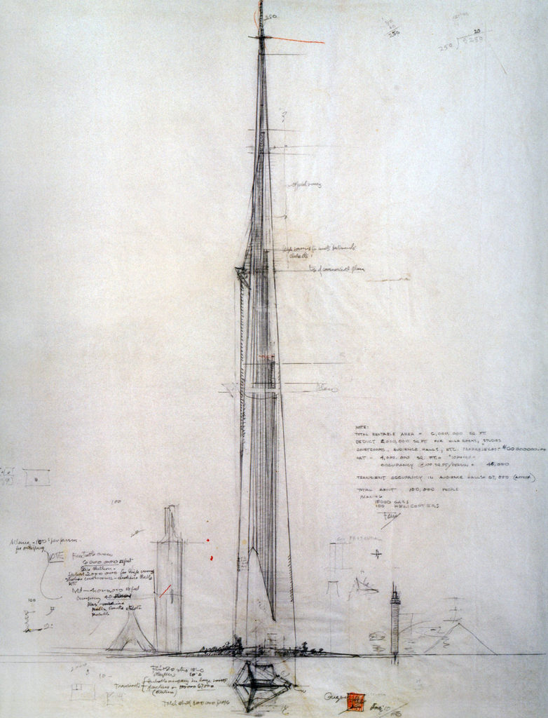
Sketch for Frank Lloyd Wright’s proposed mile high skyscraper, The Illinois. Source: Wright Mile Gallery, MCM Daily
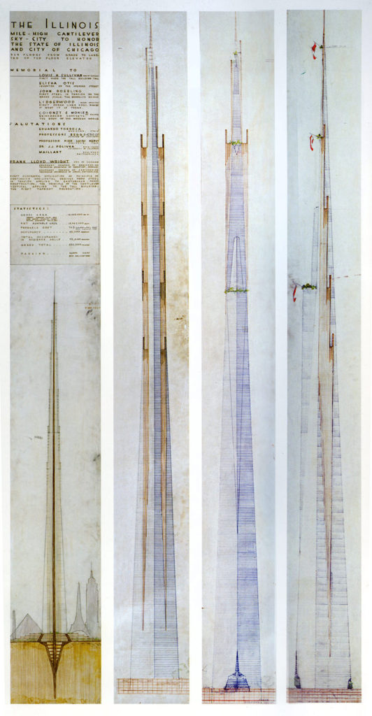
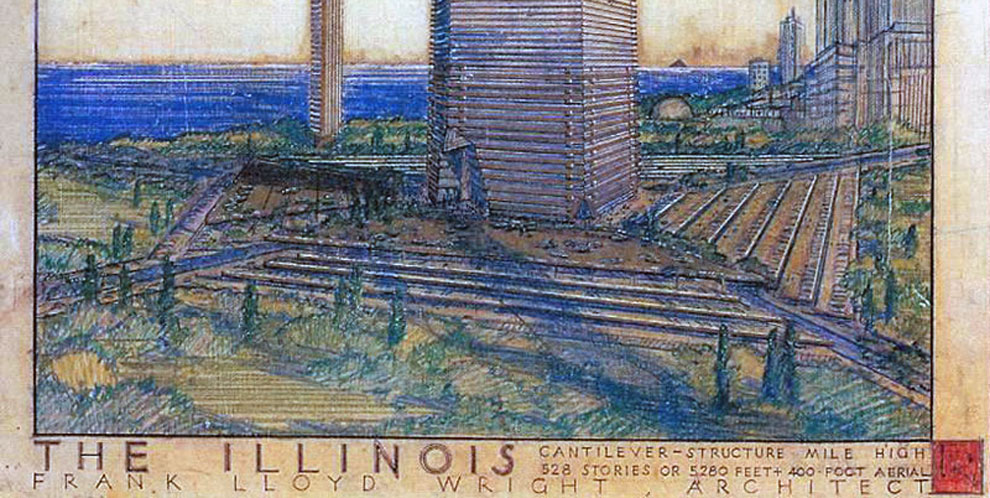
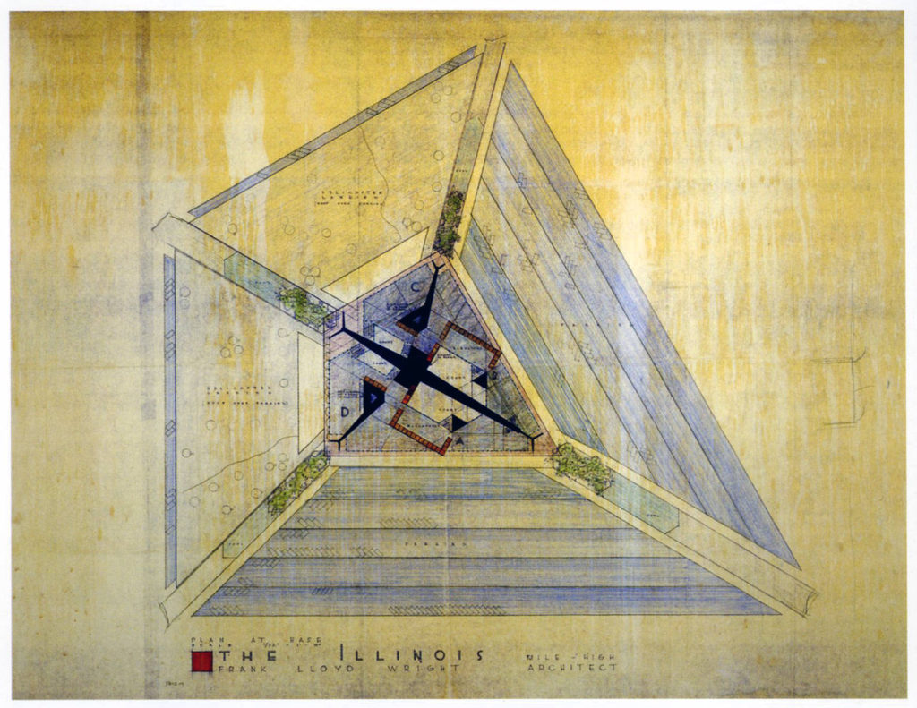
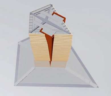
Frank Lloyd Wright illustrations of The Illinois. L to R: Cross-section; Back exterior view; Front exterior view; Side exterior view. Source: Wright Mile Gallery, MCM DailyClose-up view of the five-story base of The Illinois. Source: Frank Lloyd Wright FoundationIllustration of the footprint of The Illinois base and tower. Source: Source: Wright Mile Gallery, MCM DailyFrank Lloyd Wright illustration of The Illinois, showing the five-story base structure and the transition of the central reinforced concrete core into the “taproot” foundation structure. In the background are scale silhouettes of famous tall structures: Eiffel Tower, the Great Pyramid, and Washington Monument. Source: Wright Mile Gallery, MCM Daily
2. Tenuity, continuity and evolution of Wright’s concept for an organic high-rise building
Two aspects of Wright’s concept of organic architecture are the structural principles he termed “tenuity” and “continuity,” both of which he applied in the context of cantilevered and cable-supported structures, such as slender buildings and bridges. Author Richard Cleary reported that Wright first used the term tenuity in his 1932 book Autobiography, and offered his most succinct explanation in his 1957 book Testament.
“The cantilever is essentially steel at its most economical level of use. The principle of the cantilever in architecture develops tenuity as a wholly new human expression, a means, too, of placing all loads over central supports, thereby balancing extended load against opposite extended load.”
“This brought into architecture for the first time another principle in construction – I call it continuity – a property which may be seen as a new, elastic, cohesive, stability. The creative architect finds here a marvelous new inspiration in design. A new freedom involving far wider spacing of more slender supports.”
“Thus architecture arrived at construction from within outward rather than from outside inward; much heightening and lightening of proportions throughout all building is now economical and natural, space extended and utilized in a more liberal planning than the ancients could ever have dreamed of. This is now the prime characteristic of the new architecture called organic.”
“Construction lightened by means of cantilevered steel in tension makes continuity a most valuable characteristic of architectural enlightenment.”
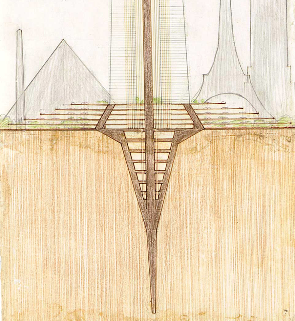
The structural principles of tenuity and continuity are manifest in Wright’s high-rise building designs that are characterized by a deep “taproot” foundation that supports a central load bearing core structure from which the individual floors are cantilevered. A cross-section of the resulting building structure has the appearance of a tree deeply rooted in the Earth with many horizontal branches.
Before looking further at the Mile-High Skyscraper, we’ll take a look at three of its high-rise predecessors and one later design, all of which shared Wright’s characteristic organic architectural features derived from the application of tenuity and continuity: taproot foundation, load-bearing core structure and cantilevered floors:
St. Mark’s Tower project
SC Johnson Research Tower
Price Tower
The Golden Beacon
St. Mark’s Tower project (St. Mark’s-in-the-Bouwerie, 1927 – 1931, not built)
Wright first proposed application of the taproot foundation, load-bearing concrete and steel core structure and cantilevered floors was in 1927 for the 15-floor St. Mark’s Tower project in New York City.
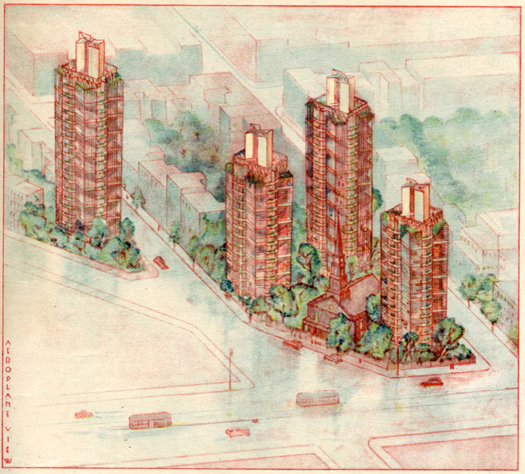
The planned St. Mark’s Tower project in the Bowery, New York City. Source: Architectural Record, 1930, via The New YorkerSt. Mark’s Tower exterior view (L) and cross-section (R) showing the central core and cantilevered floors. The deep taproot part of the foundation is not shown. Sources: (L) Architectural Record, 1930, viaThe New Yorker; (R) adapted from Frank Lloyd Wright Foundation drawing
The New York Metropolitan Museum of Modern Art (MoMA) provides this description of the St. Mark’s Tower project.
“The design of these apartment towers for St. Mark’s-in-the-Bouwerie in New York City stemmed from Wright’s vision for Usonia, a new American culture based on the synthesis of architecture and landscape. The organic “tap-root” structural system resembles a tree, with a central concrete and steel load-bearing core rooted in the earth, from which floor plates are cantilevered like branches.”
“This system frees the building of load-bearing interior partitions and supports a modulated glass curtain wall for increased natural illumination. Floor plates are rotated axially to generate variation from one level to the next and to distinguish between living and sleeping spaces in the duplex apartments.”
While the St. Mark’s Tower project was not built, this basic high-rise building design reappeared from the mid-1930s to the mid-1960s as a “city dweller’s unit” in Wright’s Broadacre City plan and was the basis for the Price Tower built in the 1950s.
SC Johnson Research Tower, Racine, WI (1943 – 1950)
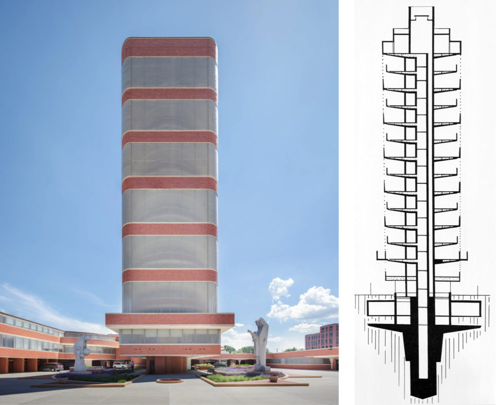
The 15-floor, 153 foot (46.6 m) tall SC Johnson Research Laboratory Tower, built between 1943 and 1950 in Racine, WI, was the first high-rise building to actually apply Wright’s organic design with a taproot foundation, load-bearing concrete and steel core structure and cantilevered floors. On their website, SC Johnson describes the structural design of this building as follows:
“One of Frank Lloyd Wright’s famous buildings, the tower rises more than 150 feet into the air and is 40 feet square. Yet at ground level, it’s supported by a base only 13 feet across at its narrowest point. As a result, the tower almost seems to hang in the air – a testament to creativity and an inspiration for the innovative products that would be developed inside.”
“Alternating square floors and round mezzanine levels make up the interior, and are supported by the “taproot” core, which also contains the building’s elevator, stairway and restrooms. The core extends 54 feet into the ground, providing stability like the roots of a tall tree.”
Because of the change in fire safety codes, and the impracticality of retrofitting the building to meet current code requirements, SC Johnson has not used the Research Tower since 1982. However, they restored the building in 2013 and now the public can visit as part of the SC Johnson Campus Tour.
You can make reservations at the following link for the Campus Tour and a separate tour of the nearby Herbert F. Johnson Prairie-style home, Wingspread, also designed by Frank Lloyd Wright: https://reservations.scjohnson.com/Info.aspx?EventID=8
Price Tower, Bartlesville, OK (1952 – 1956)
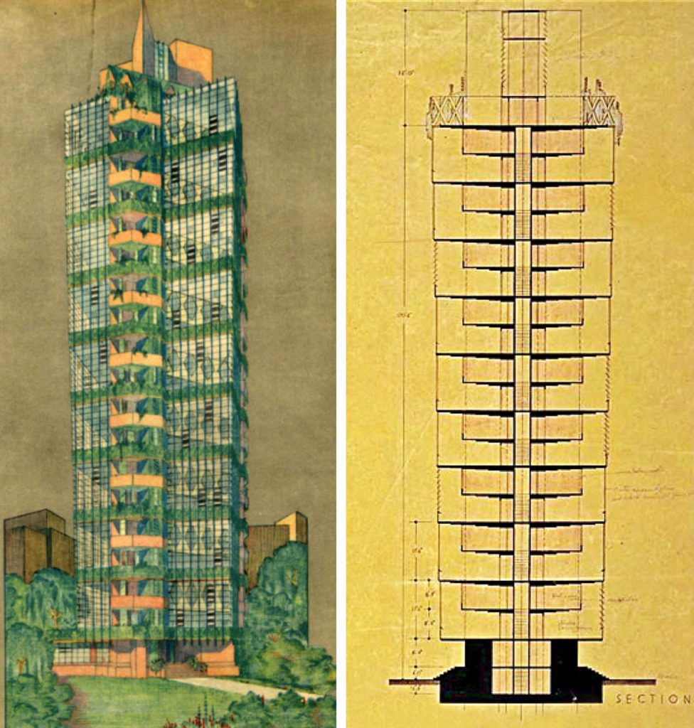
The 19-floor, 221 foot (67.4 m) tall Price Tower, completed in 1956 in Bartlesville, OK, is an evolution of Wright’s 1927 design for the St. Mark’s Tower project. Wright nicknamed the Price Tower, “the tree that escaped the crowded forest,” referring to the building’s cantilever construction and the origin of its design in a project for New York City. Price Tower also has been called the “Prairie Skyscraper.”
H.C. Price commissioned Frank Lloyd Wright to design Price Tower, which served as his corporate headquarters until 1981 when it was sold to Phillips Petroleum. Philips deemed the exterior exit staircase a safety risk and only used the building for storage until 2000, when the building was donated to the Price Tower Arts Center. Since then, Price Tower has been returned to its multi-use origins and public tours are offered, including a visit to the restored 19th floor executive office of H.C. Price and the H.C. Price Company corporate apartment with the original Wright interiors. You can arrange your tour here: https://www.pricetower.org/tour/
You also can stay at the Inn at Price Tower, which has seven guest rooms. You’ll find details here: https://www.pricetower.org/stay/
The Golden Beacon, Chicago, IL (1959, not built)
The Golden Beacon was a concept for a 50-floor mixed-use office and residential apartment building in Chicago, IL.
The Golden Beacon exterior view (L), cross-section showing taproot foundation, central core and cantilever floors. (R). Sources: (L) https://stoutbooks.com/, (R) Richard Cleary, “Lessons in Tenuity….”
As shown in the cross-section diagram, the building design followed Wright’s practice with a deep taproot foundation, a central load-bearing core and cantilevered floors. This design is very similar to the foundation structure proposed for the earlier Mile-High Skyscraper.
The Golden Beacon exterior view. Source: Frank Lloyd Wright Foundation via https://treedowntown.com/
3. Extrapolating to the Mile-High Skyscraper
By 1956, Wright’s characteristic organic architectural features for high-rise buildings, derived from the application of tenuity and continuity, had only appeared in two completed high-rise buildings, the 15-floor SC Johnson Laboratory Tower and the 19-floor Price Tower. These two important buildings demonstrated the practicality of the taproot foundation, load-bearing concrete and steel core structure and cantilevered floors for tall, slender buildings. With the unveiling of The Illinois, Wright made a remarkable extrapolation of these architectural principles in his conceptual design of this breathtaking 528 floor, 5,280 feet (1,609 meters) tall skyscraper.
Blaire Kamin, writing for the Chicago Tribune in 2017, reported: “The Mile-High didn’t simply aim to be tall. It was the ultimate expression of Wright’s “taproot” structural system, which sank a central concrete mast deep into the ground and cantilevered floors from the mast. In contrast to a typical skyscraper, in which same-size floors are piled atop one another like so many pancakes, the taproot system lets floors vary in size, opening a high-rise’s interior and letting space flow between floors.”
In addition to the central core to support the building’s dead loads, The Illinois also incorporated an external tensioned steel tripod structure to resist external wind loads and other flexing loads (i.e., earthquakes), distributing those loads through the integral steel structure of the tripod, and resisting oscillations. In his book, “Testament,” Wright stated:
“Finally – throughout this lightweight tensilized structure, because of the integral character of all members, loads are at equilibrium at all points, doing away with oscillations. There would be no sway at the peak of The Illinois.”
Tuned mass dampers (TMD) for reducing the amplitude of mechanical vibrations in tall buildings had not been invented when Wright unveiled his design for The Illinois in 1956. The first use of a TMD in a skyscraper did not occur until the mid-1970s, first as a retrofit to the troubled, 790 foot (241 m) tall, John Hancock building completed in 1976 in Boston, and then as original equipment in the 915 foot (279 m) tall Citicorp Tower completed in 1977 in New York City. While tenuity and continuity may have given The Illinois unparalleled structural stability, I wouldn’t be surprised if TMD technology would have been needed for the comfort of the occupants on the upper floors, three-quarters of a mile above their counterparts in the next tallest building in the world.
To handle its 100,000 occupants, The Illinois had 76 elevators that were divided into five groups, each serving a 100-floor segment of the building, with a single elevator serving only the top floors. Each elevator was a five-story unit that moved on rails and served five floors simultaneously. With the tapering, pyramidal shape of the skyscraper, the vertical elevator shaft structures eventually extended beyond the sloping exterior walls, forming protruding parapets on the sides of the building. In his 1957 book, “A Testament,” Wright said the elevators were designed to enable building evacuation within one hour, in combination with the escalators that serve the lowest five floors.
Wright alluded to the building (and the elevators) being “atomic powered,” but there were no provisions for a self-contained power plant as part of the building. The much smaller Empire State Building currently has a peak electrical demand of almost 10 megawatts (MW) in July and August after implementing energy conservation measures. Scaling on the basis of gross floor area, The Illinois could have had a peak electrical demand of about 70 MW. You’ll find more information on current Empire State Building energy usage here: https://www.esbnyc.com/sites/default/files/esb_overall_retrofit_fact_sheet_final.pdf
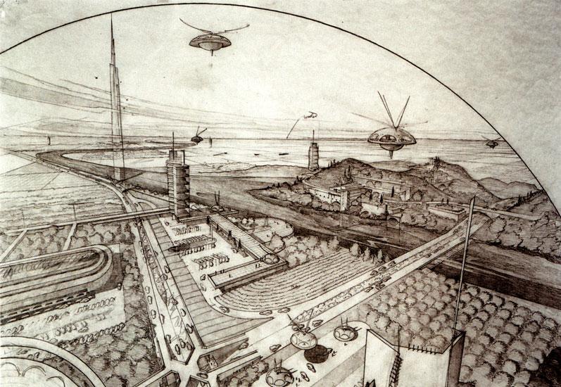
The 2012 short video by Charles Muench, “A Peaceful Day in BroadAcre City – One Mile High – Frank Lloyd Wright” (1:31 minutes), depicts The Illinois skyscraper in the spacious setting of Broadacre City and shows an animated construction sequence of the tower. Two screenshots from the video are reproduced below. You’ll find this video at the following link: https://www.dailymotion.com/video/xp86uo
Two views of the start of The Illinois construction sequence. Screenshots from Charles Muench video, 2012.
You can see more architectural details in the 2009 video, “Mile High Final Movie – Frank Lloyd Wright” (3:42 minutes), produced for the Guggenheim Museum, New York. Two screenshots are reproduced below. You’ll find the video here: https://vimeo.com/4937909
The Illinois, showing architectural exterior details. Screenshot from Guggenheim video, 2009.
The top of The Illinois, showing details at the 528th floor, including the protruding parapets for the elevators, and the 420+ foot (128 m) antenna on top. Screenshot from Guggenheim video, 2009.
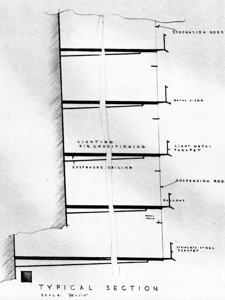
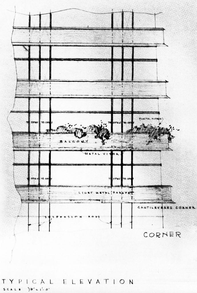
In his 1957 book, Testament, Wright provided the following two architectural drawings showing typical details of the cantilever construction of The Illinois.
The Illinois was intended for construction in a spacious setting like Broadacre City, rather than in a congested big-city downtown immediately adjacent to other skyscrapers. Two views of The Illinois in these starkly different settings are shown below.
Model of The Illinois. Source: Milwaukee Sentinel Journal
The Illinois skyscraper as part of Frank Lloyd Wright’s mid-1950s landscape for his urban planning concept known as Broadacre City. Source: utopicus2013.blogspotArtist’s concept of The Illinois skyscraper punctuating a rather congested contemporary Chicago skyline, not quite as Frank Lloyd Wright envisioned. Source: Neoman Studios
4. Wright’s Mile-High Skyscraper on Exhibit at MoMA
Since Wright’s death in 1959, his archives have been in the care of the Frank Lloyd Wright Foundation (https://franklloydwright.org/frank-lloyd-wright/) and stored at Wright’s homes / architectural schools at Taliesin in Spring Green, WI and Taliesin West, near Scottsdale, AZ.
In September 2012, Mary Louise Schumacher, writing for the Milwaukee Sentinel Journal, reported that Columbia University and the Museum of Modern Art (MoMA) in Manhattan had jointly acquired the Frank Lloyd Wright archives, which consist of architectural drawings, large-scale models, historical photographs, manuscripts, letters and other documents. You’ll find her report here: http://archive.jsonline.com/newswatch/168457936.html
Columbia University’s Avery Architectural & Fine Arts Library (https://library.columbia.edu/libraries/avery/da.html) will be the keeper of all of Wright’s paper archives, as well as interview tapes, transcripts and films. MoMA (https://www.moma.org) will add Wright’s three-dimensional models to its permanent collection.
The Frank Lloyd Wright Foundation will retain all copyright and intellectual property responsibilities for the archives, and all three organizations hope to see the archives placed online at some point in the future.
On 12 June 2017, MoMA opened its exhibit, “Frank Lloyd Wright at 150: Unpacking the Archive,” which ran thru 1 October 2017. You can take an online tour of this exhibit, which included Wright’s plans for The Illinois, here: https://www.moma.org/calendar/exhibitions/1660
MoMA’s curator of the Wright collection, Barry Bergdoll, provided an introduction to the trove of recently acquired documentation on The Illinois in a short 2017 video (4:32 minutes) at the following link: https://www.youtube.com/watch?v=VhUDu0Q08UA
Plans and sketches for The Illinois mile-high skyscraper at the 2017 MoMA exhibit. Source: MoMA
Professor Allen Sayegh with Justin Chen & John Pugh, “Mile High Final Movie – Frank Lloyd Wright” (3:42), Harvard University Graduate School of Design for the Guggenheim Museum, New York, 2009: https://vimeo.com/4937909
The Event Horizon Telescope (EHT) Collaboration reported a great milestone on 10 April 2019 when they released the first synthetic image showing a luminous ring around the shadow of the M87 black hole.
First synthetic image of the M87 black hole. Source: Event Horizon Telescope Collaboration
The bright emission ring surrounding the black hole was estimated to have an angular diameter of about 42 ± 3 μas (microarcseconds), or 1.67 ± 0.08 e-8 degrees, at a distance of 55 million light years from Earth. At the resolution of the EHT’s first black hole image, it was not possible to see much detail of the ring structure.
Significantly improved telescope performance is required to discern more detailed structures and, possibly, time-dependent behavior of spacetime in the vicinity of a black hole. The EHT Collaboration has a plan for improving telescope performance. A challenging new observational goal has been established by scientists who recently postulated the existence of a “photon ring” around a black hole. Let’s take a look at these matters.
2. Improving the performance of the EHT terrestrial observatory network
As I described in my 3 March 2017 post on the EHT, a very long baseline interferometry (VLBI) array with the diameter of the Earth (12,742 km, 1.27e+7 meters) operating in the EHT’s millimeter / submillimeter wavelength band (1.3 mm to 0.6 mm) has a theoretical angular resolution of 25 to 12 μas, with the better resolution at the shorter wavelength.
The EHT team plans to improve telescope performance in the following key areas:
Improve the resolution of the EHT
Observe at shorter wavelengths: The EHT’s first black hole image was made at a wavelength of 1.3 mm (230 GHz). Operating the telescopes in the EHT array at a shorter wavelength of 0.87 mm (frequency of 345 GHz) will improve angular resolution by about 40%. This upgrade is expected to start after 2020 and take 3 – 5 years to deploy to all EHT observatories.
Extend baselines: Adding more terrestrial radio telescopes will lengthen some observation baselines, up to the limit of the Earth’s diameter.
Improve the sensitivity of the EHT
Collect data at multiple frequencies (wide bandwidth): Black holes emit radiation at many frequencies. EHT sensitivity and signal-to-noise ratio can be improved by increasing the number of frequencies that are monitored and recorded during EHT observations. This requires multi-channel receivers and faster, more capable data processing and recording systems at all EHT observatories.
Increase the EHT aperture: The EHT team notes that the most straightforward way to boost the sensitivity of the EHT is to increase the net collecting area of the dishes in the array. You can all of the observatories participating in EHT here: https://eventhorizontelescope.org/blog/global-web-tour-eht-observatories
The size of individual radio telescopes in the EHT array vary from the 12 m Greenland Telescope with an aperture of about 113 square meters to the 50 m Large Millimeter Telescope (LMT) in Mexico with an aperture of about 2,000 square meters.
The telescope with the largest aperture is the phased ALMA array, which is comprised of up to 54 x 12 m telescopes with a effective aperture of about 7,200 square meters. The Greenland Telescope originally was a prototype for the ALMA array and was relocated to Greenland to support VLBI astronomy.
A phased array is an effective solution for VLBI observations because the requirements for mechanical precision and rigidity of the dish are easier to meet with a smaller radio telescope dish that can be manufactured in large numbers.
With higher angular resolution and improved sensitivity, and with more powerful signal processing to handle the greater volume of data, it may be possible for the EHT to “see” some detailed structures around a black hole. Multiple images of a black hole over a period of time could be used to create a dynamic set of images (i.e., a short “video”) that reveal time-dependent black hole phenomena.
3. Photon ring: New insight into the fine structure in the vicinity of a black hole
On 18 March 2020, a team of scientists postulated the existence of a “photon ring” closely orbiting a black hole. The scientists further postulated that the “glow” from the first few photon sub-rings may be directly observable with a VLBI array like the EHT.
Time-averaged results of computer simulations of the photon ring surrounding the M87 black hole. Source: Michael Johnson, et al., 18 March 2020
The abstract and part of the summary of the paper are reproduced below.
Abstract: “The Event Horizon Telescope image of the supermassive black hole in the galaxy M87 is dominated by a bright, unresolved ring. General relativity predicts that embedded within this image lies a thin “photon ring,” which is composed of an infinite sequence of self-similar subrings that are indexed by the number of photon orbits around the black hole. The subrings approach the edge of the black hole “shadow,” becoming exponentially narrower but weaker with increasing orbit number, with seemingly negligible contributions from high-order subrings. Here, we show that these subrings produce strong and universal signatures on long interferometric baselines. These signatures offer the possibility of precise measurements of black hole mass and spin, as well as tests of general relativity, using only a sparse interferometric array.”
Summary: “In summary, precise measurements of the size, shape, thickness, and angular profile of the nth photon subring of M87 and Sgr A* may be feasible for n = 1 (the first ring) using a high-frequency ground array or low Earth orbits, for n = 2 (the second ring) with a station on the Moon, and for n = 3 (the third ring) with a station in L2 (Lagrange Point).”
Five Lagrange points in the Earth-Sun system. L2 is behind the Earth. Source: NASA
The complete, and quite technical, 18 March 2020 paper by Michael Johnson, et al., “Universal interferometric signatures of a black hole’s photon ring,” is available on the Science Advances website here: https://advances.sciencemag.org/content/6/12/eaaz1310
4. EHT images black hole-powered relativistic jets
On 7 April, 2020, the EHT Collaboration reported that it had produced images with the finest detail ever seen of relativistic jets produced by a supermassive black hole. The target of their observation was Quasar 3C 279, which contains a black hole about one billion times more massive than our Sun, and is about 5 billion light-years away from Earth in the constellation Virgo.
With a resolution of 20 μas (microarcseconds) for observations at a wavelength of 1.3 mm, the EHT imaging revealed that two relativistic jets existed. As shown in the following figure, lower resolution imaging by the Global 3mm VLBI Array (GMVA) and a VLBI array observing at 7 mm wavelength did not show two distinct jets.
Illustration of multi-wavelength 3C 279 jet structure in April 2017. The observing dates, arrays, and wavelengths are noted at each panel. Source: J.Y. Kim (MPIfR), Boston University Blazar Program (VLBA and GMVA), and Event Horizon Telescope Collaboration
In their 7 April 2020 press release, the EHT Collaboration reported: “For 3C 279, the EHT can measure features finer than a light-year across, allowing astronomers to follow the jet down to the accretion disk and to see the jet and disk in action. The newly analyzed data show that the normally straight jet has an unexpected twisted shape at its base and revealing features perpendicular to the jet that could be interpreted as the poles of the accretion disk where the jets are ejected. The fine details in the images change over consecutive days, possibly due to rotation of the accretion disk, and shredding and infall of material, phenomena expected from numerical simulations but never before observed.”
Time-dependent behavior of the two relativistic jets from Quasar 3C 279. Source: Screenshot from Event Horizon Telescope Collaboration video
The following short video (1:14 minutes) from the EHT Collaboration shows the 3C 279 quasar jets and their motion over the course of one week, from 5 April to 11 April 2017, as observed by the EHT.
5. Adding space-based EHT observatories
Imaging the M87 photon ring will be a challenging goal for future observations with an upgraded EHT. As indicated in the paper by Michael Johnson, et al., an upgraded terrestrial EHT array may be able to “see” the first photon sub-ring. However, space-based telescopes will be needed to significantly extend the maximum 12,742 km (7,918 miles) baseline of the terrestrial EHT array and provide a capability to image the photon ring in greater detail.
Here’s how the EHT terrestrial baseline would change with space-based observatories:
Low Earth orbit (LEO): Add 370 – 460 km (230 – 286 miles) for a single telescope in an orbit similar to the International Space Station
Geosynchronous orbit: Add 35,786 km (22,236 mi) for a single telescope, or up to twice that for multiple telescopes
Moon: Add Earth-Moon average distance: 384,472 km (238,900 miles)
L2 Lagrange point: Add about 1.5 million km (932,057 miles)
It seems to me that several EHT observatories in geosynchronous orbits could be a good solution that could be implemented sooner than an observatory on the Moon or at L2. Geosynchronous telescopes would greatly expand the EHT baseline and the spacecraft could make long observing runs from orbital positions that are relatively fixed in relation to the terrestrial EHT sites. In-orbit servicing would be more practical in geosynchronous orbit than at L2. In February 2020, Northrop-Grumman demonstrated the ability to remotely restore a large communications satellite that was running out of fuel in geosynchronous orbit. With remote servicing, a geosynchronous observatory could have a long operating life.
6. In conclusion:
With the ongoing improvements to the terrestrial EHT array and its data recording and processing systems, we should see many more black hole observations reported in the years ahead. I’m looking forward to direct observation of M87’s photon ring and the first look at the Sagittarius A* black hole near the center of our Milky Way galaxy. The time delay between data acquisition (i.e., from a series of observation runs of a particular target) and reporting is about three years. This is understandable given the mass of data that must be aggregated from the many EHT observatories to synthesize images of a target black hole. Hopefully, this time delay can be shortened in the years ahead.
Within the next decade, a plan to expand the EHT array to include orbital and/or lunar observatories could be in developed. Hopefully, funding for spacecraft development and deployment will follow.
7. For more information:
See the following sources for more information on the EHT and imaging a black hole:
On a 2016 road trip to the Black Hills, I had long transit days each way on Interstate 90 through southern Minnesota and South Dakota. One thing I noticed was that many of the heavy tractor-trailers on this high speed route were modern, streamlined vehicles that used a variety of aerodynamic devices that appeared useful for reducing aerodynamic drag and fuel consumption.
These tractor-trailers are Class 8 heavy trucks with a gross vehicle weight (GVW) of greater than 33,000 pounds (14,969 kg). The maximum GVW is set on a case-by-case basis using the Federal Bridge Formula Weights published by the Department of Transportation’s (DOT) Federal Highway Administration (FHWA) at the following link: https://ops.fhwa.dot.gov/freight/publications/brdg_frm_wghts/index.htm
For example, a long 5-axle tractor-trailer, commonly called an “18-wheeler,” can have a GVW up to 85,500 pounds (38,782 kg), but it is limited to a maximum GVW of 80,000 pounds (36,287 kg) when operating on federal interstate highways. The higher weight limit may apply on other roads if permitted by state and local jurisdictions.
Class 8 Trucks make up only 4% of the vehicles on the road. However, they use about 20% of the nation’s transportation fuel. The following Department of Energy (DOE) video, entitled “Energy 101: Heavy Duty Vehicle Efficiency,” provides an introduction to what’s being done to introduce a variety of new technologies that will improve the performance and economy of Class 8 tractor-trailers while reducing their environmental impact: https://www.energy.gov/eere/videos/energy-101-heavy-duty-vehicle-efficiency
In this post, we’ll take a look at the following:
Three US and Canadian programs to improve tractor-trailer aerodynamics, fuel efficiency and freight efficiency:
US Environmental Protection Agency (EPA) SmartWay® Transport Partnership
Canadian Center for Surface Transportation Technology
US Department of Energy (DOE) SuperTruck program
The North American Council for Freight Efficiency’s (NACFE) Annual Fleet Fuel Study for 2019, which provides insights into the current state of the US Class 8 tractor-trailer fleet.
Accessories available to improve the aerodynamic efficiency of existing Class 8 tractor-trailers.
Aerodynamic Class 8 tractor-trailers from major US manufacturers, including:
Manufacturer’s flagship Class 8 trucks
Test trucks developed for the DOE SuperTruck program
Other advanced Class 8 truck designs and test trucks that are demonstrating new freight vehicle technologies.
Electric-powered Class 8 trucks that are about to enter service with the potential to revolutionize the freight trucking industry.
In the body of this post are links to 12 individual articles I’ve written on advanced Class 8 trucks, each of which can be downloaded as a pdf file. You’ll also find many other links to useful external resources.
2. US and Canadian programs to improve tractor-trailer aerodynamics and freight efficiency
Freight transportation is a cornerstone of the U.S. economy. In 2012, U.S. businesses spent $1 trillion to move $12 trillion worth of goods (8.5% of GDP). However, freight accounts for 9% of all U.S. greenhouse gas (GHG) emissions, and trucking is the dominant mode. The following programs are focused on reducing the GHG emissions of the freight trucking industry.
2.1 US SmartWay® Transport Partnership
The trucking industry’s ongoing efforts to improve heavy freight vehicle performance and economics were aided in 2004 by the creation of the SmartWay® Transport Partnership, which is administered by the Environmental Protection Agency (EPA). SmartWay® is a voluntarily program for achieving improved fuel efficiency and reducing the environmental impacts from freight transport. The goal is, “to move more freight, more miles, with lower emissions and less energy.” The SmartWay® website is at the following link: https://www.epa.gov/smartway
SmartWay® is promoting the following strategies to help the heavy trucking industry meet this goal:
Idle reduction
Speed control
Driver training
Aerodynamics
Tire technologies
Lubricants
Hybrid power trains
Improved freight logistics
Vehicle weight reduction
Intermodal freight capability
Alternative fuels
Long combination vehicles (LVCs, such as double trailers)
A truck and trailer fitted out with all the essential efficiency features can be sold as a SmartWay® “designated” model. A “designated” tractor-trailer combo can be as much as 20% more fuel-efficient than the comparable standard model.
2.2 Canadian Center for Surface Transportation Technology
In May 2012, the Canadian Center for Surface Transportation Technology (CSTT) issued technical report CSTT-HVC-TR-205, entitled, “Review of Aerodynamic Drag Reduction Devices for Heavy Trucks and Buses.” In Table 2 of this report, CSTT provides the following table showing the relative power consumption of aerodynamic drag and rolling / accessory drag as a function of vehicle speed for a representative heavy truck on a zero grade road with properly inflated tires. Results will be different for streamlined trucks that have already have taken steps to reduce aero drag.
Relative magnitude of drag components. Source: CSTT, 2012
In this example, rolling / accessory drag dominates at lower speeds typical of urban driving. At 50 mph (80 kph) aerodynamic drag and rolling / accessory drag are approximately equal. At higher speeds, aerodynamic drag dominates power consumption. The speed limit on I-90 in South Dakota typically is 80 mph (129 kph). At this speed the aero drag contribution is even higher than shown in the above table.
Key points from this CSTT report include the following:
For tractor-trailers, pressure drag is the dominant component of vehicle drag, due primarily to the large surface area facing the main flow direction and the large, low-pressure wake resulting from the bluntness of the back end of the vehicle.
Aero-tractor models can reduce pressure drag by about 30% over the boxy classic style tractor.
Friction drag occurring along the sides and top of tractor-trailers makes only a small contribution to total drag (10% or less), so these areas are not strong candidates for drag-reduction.
The gap between the tractor and the trailer has a significant effect on total drag, particularly if the gap is large. Eliminating the gap entirely could reduce total drag by about 7%.
Side skirts or underbody boxes prevent airflow from entering the under-trailer region. These types of aero devices could reduce drag by 10 – 15%.
Wind-tunnel and road tests have demonstrated that a “boat tail” with a length of 24 – 32 inches (61 – 81 cm) is optimal for reducing drag due to the turbulent low-pressure region behind the trailer.
Adding a second trailer to form a long combination vehicle (LCV), and thus doubling the freight volumetric capacity, results in a very modest increase in drag coefficient (as low as about 10%) when compared to a single trailer vehicle.
In cold Canadian climates, the aerodynamic drag in winter can be nearly 20% greater than at standard conditions, due to the ambient air density. For highway tractor-trailers, this results in about a 10% increase in fuel consumption from aerodynamic drag when compared to the reference temperature, further emphasizing the importance of aerodynamic drag reduction strategies for the Canadian climate.
SuperTruck is major DOE technology innovation program with many industry partners representing a broad segment of the US industrial base for heavy tractor-trailers. This program, run by DOE’s Vehicle Technologies Office, focused on Class 8 trucks with internal combustion engines during the first two five-year program phases known as SuperTruck 1 and 2. Program focus shifted to electric powertrains in the third five-year phase known as SuperTruck 3.
Following is an overview of the SuperTruck program. Additional sources of information are listed at the end of this post.
SuperTruck 1 (2010-2016)
The first phase, known as SuperTruck 1, was a $284 million public-private partnership in which industry matched federal grants dollar-for-dollar. Four Class 8 truck manufacturers led teams in the SuperTruck 1 program:
Freightliner (Daimler North America)
International (Navistar)
Peterbilt (teamed with Cummins)
Volvo North America
DOE SuperTruck 1 teams. Source: DOE
Objectives for the DOE SuperTruck 1 program were:
Demonstrate a 50% freight efficiency improvement from a “baseline” 2009 model year Class 8 tractor-trailer.
Freight efficiency is the product of payload weight (in tons) and fuel economy (in miles per gallon), with results reported in North America as ton-miles per gallon.
Performance would be measured with a demonstration SuperTruck operated at 65,000 pounds GVW.
Average fuel efficiency of the baseline tractors in SuperTruck 1 was 6.2 mpg.
Improve engine efficiency by 8% to achieve 50% brake thermal efficiency (BTE), and thereby boost fuel efficiency by 16%.
The BTE of an engine is the ratio of Brake Power (BP) to Fuel Power (FP).
Brake power (BP) is the amount of power available at the crankshaft, taking into account engine friction losses (i.e., between cylinder and walls, crankshaft bearing, etc.).
Fuel power (FP) is a measure of the calorific value of the fuel used to deliver a particular value of BP.
Typical Class 8 truck diesel engines operate at 41 – 43% BTE. This means that 41 – 43% of the calorific value of the fuel is converted into power available at the crankshaft. The remaining 57 – 59% of the calorific value of the fuel is lost as heat that is carried off by the engine cooling system and engine exhaust system. In some advanced engines, turbochargers and waste heat recovery systems are used to increase BTE by recovering some energy from exhaust gases.
Show pathways for a further 5% improvement in engine efficiency (to achieve a BTE of 55%).
The four SuperTrucks developed by the respective teams are described in Section 5. All teams met or exceeded the SuperTruck I objectives set by DOE.
SuperTruck 2 (2017 – 2022)
SuperTruck 2 is a five-year, $160-million public-private partnership with industry matching federal grants dollar-for-dollar. Five teams are participating in the SuperTruck 2 program:
In August 2016, DOE announced that the four teams from SuperTruck 1 would continue their participation in SuperTruck 2.
A new team led by PACCAR, with truck manufacturer Kenworth as a team member, joined SuperTruck 2 in October 2017.
Objectives for the DOE SuperTruck 2 program are:
Improve freight efficiency (ton-miles per gallon) by 100% relative to a “best in class” 2009 truck (same baseline as in SuperTruck I), with a stretch goal of 120%.
Demonstrate 55% Brake Thermal Efficiency on an engine dynamometer.
Develop technologies that are commercially cost effective in terms of a simple payback.
Michael Berube, head of DOE’s Vehicle Technologies Office, acknowledged that the SuperTruck 2 objectives are beyond what the participants think they can achieve. However, with industry receiving dollar-for-dollar federal grants, Berube said, “…the program will allow them to try higher-risk technologies than they might on their own.”
Among the candidate technologies for SuperTruck 2 are:
Engines with waste heat recovery
Various forms of hybrid diesel-electric systems
More radical aerodynamic improvements, including active devices and completely redesigned cabs.
“Think of the benefit to the industry and to the country if they can meet that goal of doubling freight efficiency. There are 1.7 (to 2.5) million Class 8 trucks out there, each traveling an average of 66,000 miles a year. Doubling their efficiency could reduce petroleum consumption by 300 million barrels a year,” Berube said. At today’s fuel costs, that would save operators up to $20,000 per truck per year.
While most SuperTruck 2 programs wrapped up in 2022, PACCAR’s program was completed at the end of 2023 due to its later starting date.
SuperTruck 3 (2022 – 2027)
In October 2021, DOE launched a $199 million, five-year program to support the development of zero-emission vehicles, with $127 million directed to the SuperTruck 3 program, which will fund 50:50 cost-sharing projects to develop battery-electric and fuel cell medium- and heavy-duty trucks and freight system solutions with payload capacity and range equivalent to typical diesel-powered counterpart vehicles.
This DOE program includes three firms from the previous SuperTruck 2 program: PACCAR Inc., Volvo Group North America and Daimler Trucks North America.
PACCAR Inc.: $33 million in DOE cost-sharing funds to develop 18 Class 8 battery-electric vehicles with advanced batteries and a demonstration megawatt-class charging station.
Volvo Group North America: $18 million in DOE cost-sharing funds to develop a 400-mile-range Class 8 battery-electric tractor-trailer with advanced aerodynamics, electric braking, EV-optimized tires, automation and route planning. It also will develop and demonstrate a megawatt-class charging station.
Daimler Trucks North America: $26 million in DOE cost-sharing funds to develop and demonstrate two Class 8 hydrogen fuel cell trucks with a 600-mile range and 25,000-hour durability.
In addition, the SuperTruck 3 program includes Ford Motor Company and General Motors, both of which will focus on smaller freight vehicles, up to Class 6 Super Duty trucks.
3. The NACFE Annual Fleet Fuel Study
The North American Council for Freight Efficiency (NACFE) (https://nacfe.org/) describes its mission as working to “drive the development and adoption of efficiency enhancing, environmentally beneficial, and cost-effective technologies, services and methodologies in the North American freight industry.”
One of NACFE’s important products is the Annual Fleet Fuel Study, which reports on the adoption of 85 technologies and practices for improving freight efficiency among major North American Class 8 truck fleets operators. The 2019 Annual Fleet Fuel Study was based on data from 21 fleets operating 73,844 tractors and 239,292 trailers. You can download the NACFE 2019 Annual Fleet Fuel Survey here: https://nacfe.org/annual-fleet-fuel-studies/
The following chart shows adoption rates among NACFE member fleets in seven technology categories. Tractor aerodynamic improvements (light blue line) have a high rate of adoption, at about 62% in 2018. In contrast, trailer aerodynamic improvements (purple line) have a much lower rate of adoption, at about 25% in 2018.
Source: NACFE 2019 Annual Fleet Fuel Study
The Annual Fleet Fuel Study includes an analysis of the average fuel economy delivered by the combined Class 8 tractor-trailer fleet. Over the 16 years of this study, the average year-on-year improvement in fuel economy has been 2.0%. Fuel economy results are summarized in the following chart.
Source: NACFE 2019 Annual Fleet Fuel Study
Key points in this chart are:
The blue line represents the average fuel economy of the NACFE fleet from 2003 to 2018. In 2018, the NACFE fleet-wide average fuel economy increased to 7.27 mpg.
The red line is a hypothetical “business as usual” case, which is an estimate of what NACFE fleet fuel economy would be based only on improvements in engine efficiency. In 2018, “business as usual” would have yielded 6.37 mpg.
The difference between the blue and red curves represents the fuel efficiency improvements attributable to all other technologies and practices. In 2018, that difference was 0.9 mpg, meaning that actual performance was 14% better than the “business as usual” case.
The lowest (purple) curve is based on actual data reported to the U.S. Department of Transportation’s Federal Highway Administration (FHWA) for the approximately 2.5 million over-the-road tractor-trailers operating in the US. This average fleet fuel efficiency in 2017 was 5.98 mpg, well behind the fuel efficiency performance reported by NACFE fleet operators (which is included in the FHWA data).
4. Accessories available to improve the aerodynamic efficiency of existing tractor-trailers
The typical big rig has an aerodynamic drag coefficient, CD, of over 0.6, which has a huge effect on fuel economy, particularly during high-speed highway driving. Many truck manufacturers and third-party firms offer add-on kits with a variety of devices that can be installed on an existing tractor-trailer to improve its aerodynamic efficiency. Here we’ll look at a few of those devices:
Trailer tails (tapered boat-tails on the back of the trailer)
Trailer skirts
Aerodynamic wheel covers
The U.S. firm STEMCO (http://www.stemco.com) offers two aero kits for improving conventional tractor-trailer aerodynamics:
TrailerTail®, which is installed at the back of the trailer, reduces the magnitude of the turbulent low-pressure area that forms behind the trailer at high speeds.
EcoSkirt®, which is installed under the trailer, reduces aerodynamic drag under the trailer where air hits the trailer’s rear axles. The side fairings streamline and guide the air around the sides and to the back of the trailer.
Both of these aerodynamic devices are shown in the following figure. This was a tractor-trailer configuration that I saw frequently on I-90.
Source: STEMCO
STEMCO allocates the primary sources of tractor-trailer aerodynamic drag as shown in the following figure.
Source: STEMCO
STEMCO claims the following benefits from their aero kits:
“TrailerTail® fuel savings complement other aerodynamic technologies.”
“A TrailerTail® reduces aerodynamic drag by over 12% equating to over 5% fuel efficiency improvement at 65 mph (105 kph) and over 12% fuel efficiency improvement when combined with STEMCO’s side skirts and other minor trailer modifications.”
STEMCO TrailerTail® meets the SmartWay® advanced trailer end fairings criteria for a minimum of 5% fuel savings and the STEMCO EcoSkirt® meets the advanced trailer skirts qualifications with greater than 5% fuel savings. The payback period for these aero devices is expected to be about one year.
You’ll find more details on STEMCO’s tractor-trailer drag reduction products, including a short “Aerodynamics 101” video, at the following link: http://www.stemco.com/aero-u/
More details on TrailerTail®, including its automatic deployment and operational use, are shown in a short video at the following link: https://www.youtube.com/watch?v=qPrM3-CCth8
Another firm, Aerotech Caps, offers a range of aero kits for improving truck aerodynamics, including aerodynamic wheel covers, aerodynamic trailer skirts, tail fairings and vortex generators. You can see their product line at the following link: https://aerotechcaps.com/#aerotechcaps
Source: Aerotech Caps
Aerotech Caps claims that its aerodynamic wheel covers deliver about 2.4% increased miles per gallon when installed on rear tractor and all trailer wheels. Payback period for this aero kit is expected to be about one year.
5. Aerodynamic Class 8 production tractor-trailers and SuperTrucks from major US manufacturers
Conventional, top-of-the-line tractor-trailers on the market today have significantly improved aerodynamic and fuel efficiency performance in comparison to their predecessors. The aero gains have been achieved by integrating many of the aero features described above into the basic designs for the latest Class 8 tractor-trailers on the market. In addition, optional aero kits are available to further improve performance.
Class 8 truck manufacturers’ market share in the U.S. as of December 2019 is shown in the following chart.
Note that Freightliner is a Daimler North America brand along with Western Star. Peterbilt and Kenworth are PACCAR brands. International is a Navistar brand and Mack is a Volvo brand.
Now we’ll take a look at the most aerodynamic tractor-trailers offered in 2020 by the top five manufacturers in the US Class 8 truck market. Collectively, these manufacturers account for almost 90% of the US Class 8 heavy truck market.
Four of the five top manufacturers, Freightliner, Peterbilt, International and Volvo, led teams in the DOE SuperTruck 1 program (2010-2016) and are continuing their participation in the SuperTruck 2 program (2017 – 2022). Kenworth did not participate in SuperTruck 1, but did participate in SuperTruck 2 as a member of a new team led by their parent firm, PACCAR.
You’ll find my articles on these tractor-trailers at the following links:
6. Other advanced Class 8 tractor-trailer designs and test trucks
The future of heavy freight vehicles is certain to include increasingly aerodynamic tractor-trailers with more efficient diesel and hybrid powertrains. While the five teams participating in the DOE SuperTruck program are demonstrating significantly improved Class 8 tractor-trailer performance, other firms have been working in parallel to develop their own advanced truck concepts and test trucks. In this section, we’ll take a look at the following advanced integrated tractor-trailers.
You’ll find my articles at these tractor-trailers at following links:
7. Advanced electric-powered Class 8 tractor-trailers
A variety of electric-powered heavy trucks and tractor trailers are being developed for the worldwide market and several are being operationally tested. The most common electric energy sources are be battery-electric or hydrogen fuel cell + battery.
“Battery electric vehicles are around 90% efficient with the electricity that flows into the charger when it is converted into motion by the onboard motors.”
“Hydrogen fuel cell vehicles are understandably less efficient, using the source electricity to break apart water, compress it, transfer it into the vehicle, and then convert the hydrogen back into electricity by combining it with ambient oxygen. Estimates for the efficiency of the electricity used to produce hydrogen, then get converted back to electricity in fuel cell vehicles, is around 40%.”
Lithium-ion batteries currently are the dominant type of battery used in electric vehicles. Boston Consulting Group reported that one particular type, the lithium nickel-manganese-cobalt (NMC) battery, has good overall performance, excels on specific energy, has the lowest self-heating rate, and is a preferred candidate for electric vehicles. For more information, see the 10 July 2019 Battery University article, “BU-205: Types of Lithium-ion Batteries,” at the following link: https://batteryuniversity.com/learn/article/types_of_lithium_ion
While less efficient in overall energy conversion, the hydrogen fuel cell weighs much less and can store much more energy than a comparably-sized, current-generation battery packaged for a heavy-duty truck application. For more information on hydrogen fuel cells, see the May 2017 University of California (UC) Davis presentation, “Fuel Cells and Hydrogen in Long-Haul Trucks,” at the following link: https://steps.ucdavis.edu/wp-content/uploads/2017/05/Andy-Burke-Hydrogen-Fuel-Cell-Trucks.pdf
In 2020, several heavy-duty electric truck designs are adaptations of existing Class 8 tractor-trailers with all-new electric powertrains. Examples are shown in the following table.
Some designs in 2020 were “clean-sheet” advanced electric-powered Class 8 tractor-trailers that also may offer a future path toward autonomous vehicle operation. Examples include:
Then there are even more advanced electric-powered heavy trucks that are designed originally as autonomous freight haulers without provisions for a driver’s cab. For example:
You can get a good overview of the current state of electric-powered heavy truck development in the following October 2019 video by Automotive Territory: “10 All-Electric Trucks and Freighters Showcasing the Future of Cargo Vehicles” (11:17 minutes): https://www.youtube.com/watch?v=smAleMBEszs
In this section, we’ll take a look at the “clean-sheet” advanced electric-powered Class 8 tractor-trailers. You’ll find my articles at these tractor-trailers at following links:
The DOE-sponsored SuperTruck 3 program initiated in 2022, which is funding work to develop battery-electric and fuel cell medium- and heavy-duty trucks and freight system solutions, is not funding any of the above three companies.
8. Conclusions:
Freight currently accounts for 9% of all U.S. greenhouse gas (GHG) emissions, and trucking is the dominant mode. The gradual phase-in of tractor-trailers with refined aerodynamics and diesel engines is improving fleet-wide fuel economy and thereby helping to decrease the carbon footprint of long-haul trucking.
Large improvements in freight efficiency (the product of payload weight in tons and fuel economy in miles per gallon; ton-miles per gallon) were demonstrated during the DOE SuperTruck 1 program, and greater gains are expected in SuperTruck 2, which continued into 2023. In the meantime, truck manufacturers are implementing SuperTruck technologies in their production model tractor-trailers. This is a significant step in the right direction.
With the introduction of electric-powered tractor-trailers in the next decade, the trucking industry has an opportunity to revolutionize its operations by deploying fleets of zero-emission trucks. The very aerodynamic, electric-powered Tesla Semi and the smaller freight vehicles being developed by Xos seem to be good first steps in starting the electric freight revolution. They will be joined by other electric-powered tractor-trailers and smaller freight vehicles being developed under the DOE SuperTruck 3 program, which will run thru 2027.
For the electric-powered trucks to compete effectively with diesel and hybrid-powered truck, the truck manufacturers and the freight industry needs to support deployment of the diverse nation-wide infrastructures for very-high capacity battery recharging and hydrogen refueling. With these new infrastructures in place, electric-powered freight operations can become routine and make a big contribution to reducing GHG emissions and the environmental impact of the nation’s freight hauling industry.
In spite of all of these opportunities for improving heavy tractor-trailer performance, there always will be cases when few of these are actually practical. As evidence, I offer the following photo taken at 80 mph on I-90 in South Dakota during my 2016 road trip. How do you optimize that giant drag coefficient?
National Academies report: “Review of the 21st Century Truck Partnership: Third Report,”, particularly Chapter 8, “SuperTruck,” 2015; https://www.nap.edu/download/21784
“NETL Project Partner Daimler Truck North America Debuts Next Level of Freight Efficiency with the Freightliner SuperTruck II,” National Energy Technology Laboratory press release, 3 August 2023: https://netl.doe.gov/node/12767
This post contains links to many free virtual tours and other online resources that may be of interest to you. Also check out the long list of recommended external links on the introductory webpage for Pete’s Lynx, here:
Here you’ll find virtual tours and online collections from many partner museums and other organizations. So many, that I suggest that you try finding something of interest in the “A-Z” view. There are 145 “A’s” and 8 “Z’s,” with more than 2,500 other museums and collections in between. Start at the following link: https://artsandculture.google.com/partner
2. MCN’s Ultimate Guide to Virtual Museum Resources, E-Learning, and Online Collections
On 14 March 2020, MCN (formerly the Museum Computer Network) posted “The Ultimate Guide to Virtual Museum Resources, E-Learning, and Online Collections,” at the following link: http://mcn.edu/a-guide-to-virtual-museum-resources/
This is a very extensive list of free online resources and their links. MCN notes, “This list will be continually updated with examples of museum and museum-adjacent virtual awesomeness. It is by no means exhaustive….. Every resource is free to access and enjoy.”
Architect of the Capitol – Virtual Capitol (US Capitol complex), Washington D.C.: https://www.capitol.gov
Getty, Los Angeles, CA: The Getty Search Gateway allows users to search across several of the Getty repositories, including almost 15,000 images recently placed in the public domain: https://search.getty.edu/gateway/about.html
Visit Milosh Kitchovitch’s “Amazing Places on Our Planet” YouTube channel, where you’ll find 180+ videos in 4K Ultra HD quality, and about 80 more HD videos. These videos present the places in a natural way, like you would see them if you were visiting. Here are a few examples of what you’ll find:
Virtual Visit Tours – 360 degree photographic visits to many sites in Ireland, including the two examples listed below: https://www.virtualvisittours.com
Check out the Internet Archive, which is a non-profit library of millions of free books, movies, software, music, websites, and more. The main website is here: https://archive.org. Direct links to some of the specific parts of the Internet Archive are here:
The best free cultural & educational media on the web, with more than 1,500 free online courses from top universities, 1,150 free movies, 700 free audio books, 800 free eBooks, 300 free language lessons, 15,000+ free Golden Age comics from the Digital Comic Museum, and more: http://www.openculture.com/freeonlinecourses
Biodiversity Heritage Library (BHL): This is an open-access digital archive that preserves images and documents related to botany, wildlife and biodiversity. More than 150,000 such artworks are freely available for download here: https://www.biodiversitylibrary.org
New York Public Library digital collections: Explore 890,000 items digitized from The New York Public Library’s collections. This site is a living database with new materials added every day, featuring prints, photographs, maps, manuscripts, streaming video, and more: https://digitalcollections.nypl.org
Other authors have provided similar information in the recent articles listed below. Many of the museums listed in the following articles are accessible via the Google Arts & Culture portal.