Peter Lobner
What is space weather?
Space weather is determined largely by the variable effects of the Sun on the Earth’s magnetosphere. The basic geometry of this relationship is shown in the following diagram, with the solar wind always impinging on the Earth’s magnetic field and transferring energy into the magnetosphere. Normally, the solar wind does not change rapidly, and Earth’s space weather is relatively benign. However, sudden disturbances on the Sun produce solar flares and coronal holes that can cause significant, rapid variations in Earth’s space weather.
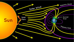 Source: http://scijinks.jpl.nasa.gov/aurora/
A solar storm, or geomagnetic storm, typically is associated with a large-scale magnetic eruption on the Sun’s surface that initiates a solar flare and an associated coronal mass ejection (CME). A CME is a giant cloud of electrified gas (solar plasma.) that is cast outward from the Sun and may intersect Earth’s orbit. The solar flare also releases a burst of radiation in the form of solar X-rays and protons.
The solar X-rays travel at the speed of light, arriving at Earth’s orbit in 8 minutes and 20 seconds. Solar protons travel at up to 1/3 the speed of light and take about 30 minutes to reach Earth’s orbit. NOAA reports that CMEs typically travel at a speed of about 300 kilometers per second, but can be as slow as 100 kilometers per second. The CMEs typically take 3 to 5 days to reach the Earth and can take as long as 24 to 36 hours to pass over the Earth, once the leading edge has arrived.
If the Earth is in the path, the X-rays will impinge on the Sun side of the Earth, while charged particles will travel along magnetic field lines and enter Earth’s atmosphere near the north and south poles. The passing CME will transfer energy into the magnetosphere.
Solar storms also may be the result of high-speed solar wind streams (HSS) that emanate from solar coronal holes (an area of the Sun’s corona with a weak magnetic field) with speeds up to 3,000 kilometers per second. The HSS overtakes the slower solar wind, creating turbulent regions (co-rotating interaction regions, CIR) that can reach the Earth’s orbit in as short as 18 hours. A CIR can deposit as much energy into Earth’s magnetosphere as a CME, but over a longer period of time, up to several days.
Solar storms can have significant effects on critical infrastructure systems on Earth, including airborne and space borne systems. The following diagram highlights some of these vulnerabilities.
 Effects of Space Weather on Modern Technology. Source: SpaceWeather.gc.ca
Characterizing space weather
The U.S. National Oceanic and Atmospheric Administration (NOAA) Space Weather Prediction Center (SWPC) uses the following three scales to characterize space weather:
- Geomagnetic storms (G): intensity measured by the “planetary geomagnetic disturbance index”, Kp, also known as the Geomagnetic Storm or G-Scale
- Solar radiation storms (S): intensity measured by the flux level of ≥ 10 MeV solar protons at GEOS (Geostationary Operational Environmental Satellite) satellites, which are in synchronous orbit around the Earth.
- Radio blackouts (R): intensity measured by flux level of solar X-rays at GEOS satellites.
Another metric of space weather is the Disturbance Storm Time (Dst) index, which is a measure of the strength of a ring current around Earth caused by solar protons and electrons. A negative Dst value means that Earth’s magnetic field is weakened, which is the case during solar storms.
A single solar disturbance (a CME or a CIR) will affect all of the NOAA scales and Dst to some degree.
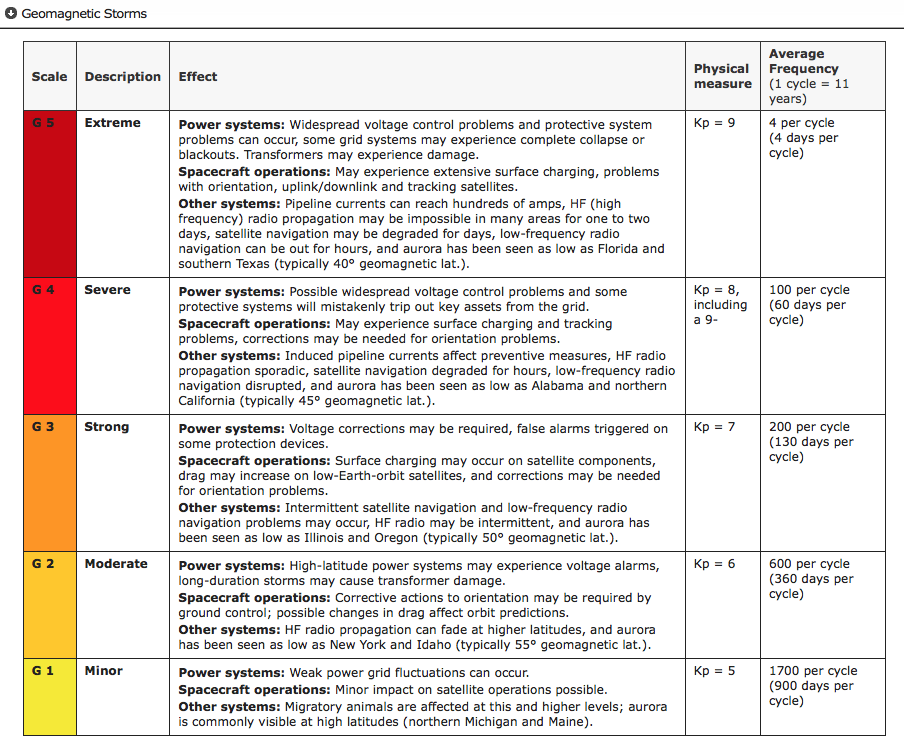
As shown in the following NOAA table (click on table to enlarge), the G-scale describes the infrastructure effects that can be experienced for five levels of geomagnetic storm severity. At the higher levels of the scale, significant infrastructure outages and damage are possible.

There are similar tables for Solar Radiation Storms and Radio Blackouts on the NOAA SWPC website at the following link:
http://www.swpc.noaa.gov/noaa-scales-explanation
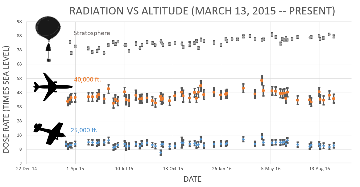
Another source for space weather information is the spaceweather.com website, which contains some information not found on the NOAA SWPC website. For example, this website includes a report of radiation levels in the atmosphere at aviation altitudes and higher in the stratosphere. In the following chart, “dose rates are expressed as multiples of sea level. For instance, we see that boarding a plane that flies at 25,000 feet exposes passengers to dose rates ~10x higher than sea level. At 40,000 feet, the multiplier is closer to 50x.”
 Source: spaceweather.com
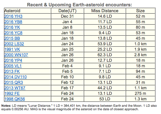
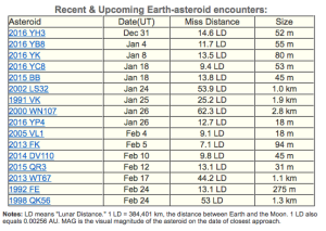
You’ll also find a report of recent and upcoming near-Earth asteroids on the spaceweather.com website. This definitely broadens the meaning of “space weather.” As you can seen the in the following table, no close encounters are predicted over the next two months.
In summary, the effects of a solar storm may include:
- Interference with or damage to spacecraft electronics: induced currents and/or energetic particles may have temporary or permanent effects on satellite systems
- Navigation satellite (GPS, GLONASS and Galileo) UHF / SHF signal scintillation (interference)
- Increased drag on low Earth orbiting satellites: During storms, currents and energetic particles in the ionosphere add energy in the form of heat that can increase the density of the upper atmosphere, causing extra drag on satellites in low-earth orbit
- High-frequency (HF) radio communications and low-frequency (LF) radio navigation system interference or signal blackout
- Geomagnetically induced currents (GICs) in long conductors can trip protective devices and may damage associated hardware and control equipment in electric power transmission and distribution systems, pipelines, and other cable systems on land or undersea.
- Higher radiation levels experienced by crew & passengers flying at high latitudes in high-altitude aircraft or in spacecraft.
For additional information, you can download the document, “Space Weather – Effects on Technology,” from the Space Weather Canada website at the following link:
http://ftp.maps.canada.ca/pub/nrcan_rncan/publications/ess_sst/292/292124/gid_292124.pdf
Historical major solar storms
The largest recorded geomagnetic storm, known as the Carrington Event or the Solar Storm of 1859, occurred on 1 – 2 September 1859. Effects included:
- Induced currents in long telegraph wires, interrupting service worldwide, with a few reports of shocks to operators and fires.
- Aurorea seen as far south as Hawaii, Mexico, Caribbean and Italy.
This event is named after Richard Carrington, the solar astronomer who witnessed the event through his private observatory telescope and sketched the Sun’s sunspots during the event. In 1859, no electric power transmission and distribution system, pipeline, or cable system infrastructure existed, so it’s a bit difficult to appreciate the impact that a Carrington-class event would have on our modern technological infrastructure.
A large geomagnetic storm in March 1989 has been attributed as the cause of the rapid collapse of the Hydro-Quebec power grid as induced voltages caused protective relays to trip, resulting in a cascading failure of the power grid. This event left six million people without electricity for nine hours.
A large solar storm on 23 July 2012, believed to be similar in magnitude to the Carrington Event, was detected by the STEREO-A (Solar TErrestrial RElations Observatory) spacecraft, but the storm passed Earth’s orbit without striking the Earth. STEREO-A and its companion, STEREO-B, are in heliocentric orbits at approximately the same distance from the Sun as Earth, but displaced ahead and behind the Earth to provide a stereoscopic view of the Sun.
You’ll find a historical timeline of solar storms, from the 28 August 1859 Carrington Event to the 29 October 2003 Halloween Storm on the Space Weather website at the following link:
http://www.solarstorms.org/SRefStorms.html
Risk from future solar storms
A 2013 risk assessment by the insurance firm Lloyd’s and consultant engineering firm Atmospheric and Environmental Research (AER) examined the impact of solar storms on North America’s electric grid.
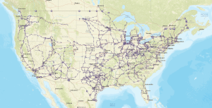 U.S. electric power transmission grid. Source: EIA
Here is a summary of the key findings of this risk assessment:
- A Carrington-level extreme geomagnetic storm is almost inevitable in the future. Historical auroral records suggest a return period of 50 years for Quebec-level (1989) storms and 150 years for very extreme storms, such as the Carrington Event (1859).
- The risk of intense geomagnetic storms is elevated near the peak of the each 11-year solar cycle, which peaked in 2015.
- As North American electric infrastructure ages and we become more dependent on electricity, the risk of a catastrophic outage increases with each peak of the solar cycle.
- Weighted by population, the highest risk of storm-induced power outages in the U.S. is along the Atlantic corridor between Washington D.C. and New York City.
- The total U.S. population at risk of extended power outage from a Carrington-level storm is between 20-40 million, with durations from 16 days to 1-2 years.
- Storms weaker than Carrington-level could result in a small number of damaged transformers, but the potential damage in densely populated regions along the Atlantic coast is significant.
- A severe space weather event that causes major disruption of the electricity network in the U.S. could have major implications for the insurance industry.
The Lloyds report identifies the following relative risk factors for electric power transmission and distribution systems:
- Magnetic latitude: Higher north and south “corrected” magnetic latitudes are more strongly affected (“corrected” because the magnetic North and South poles are not at the geographic poles). The effects of a major storm can extend to mid-latitudes.
- Ground conductivity (down to a depth of several hundred meters): Geomagnetic storm effects on grounded infrastructure depend on local ground conductivity, which varies significantly around the U.S.
- Coast effect: Grounded systems along the coast are affected by currents induced in highly-conductive seawater.
- Line length and rating: Induced current increases with line length and the kV rating (size) of the line.
- Transformer design: Lloyds noted that extra-high voltage (EHV) transformers (> 500 kV) used in electrical transmission systems are single-phase transformers. As a class, these are more vulnerable to internal heating than three-phase transformers for the same level of geomagnetically induced current.
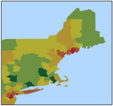
Combining these risk factors on a county-by-county basis produced the following relative risk map for the northeast U.S., from New York City to Maine. The relative risk scale covers a range of 1000. The Lloyd’s report states, “This means that for some counties, the chance of an average transformer experiencing a damaging geomagnetically induced current is more than 1000 times that risk in the lowest risk county.”
 Relative risk of power outage from geomagnetic storm. Source: Lloyd’s
You can download the complete Lloyd risk assessment at the following link:
https://www.lloyds.com/news-and-insight/risk-insight/library/natural-environment/solar-storm
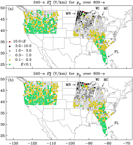
In May 2013, the United States Federal Energy Regulatory Commission issued a directive to the North American Electric Reliability Corporation (NERC) to develop reliability standards to address the impact of geomagnetic disturbances on the U.S. electrical transmission system. One part of that effort is to accurately characterize geomagnetic induction hazards in the U.S. The most recent results were reported in the 19 September 2016, a paper by J. Love et al., “Geoelectric hazard maps for the continental United States.” In this report the authors characterize geography and surface impedance of many sites in the U.S. and explain how these characteristics contribute to regional differences in geoelectric risk. Key findings are:
“As a result of the combination of geographic differences in geomagnetic activity and Earth surface impedance, once-per-century geoelectric amplitudes span more than 2 orders of magnitude (factor of 100) and are an intricate function of location.”
“Within regions of the United States where a magnetotelluric survey was completed, Minnesota (MN) and Wisconsin (WI) have some of the highest geoelectric hazards, while Florida (FL) has some of the lowest.”
“Across the northern Midwest …..once-per-century geoelectric amplitudes exceed the 2 V/km that Boteler ……has inferred was responsible for bringing down the Hydro-Québec electric-power grid in Canada in March 1989.”
The following maps from this paper show maximum once-per-century geoelectric exceedances at EarthScope and U.S. Geological Survey magnetotelluric survey sites for geomagnetic induction (a) north-south and (b) east-west. In these maps, you can the areas of the upper Midwest that have the highest risk.
The complete paper is available online at the following link:
http://onlinelibrary.wiley.com/doi/10.1002/2016GL070469/full
Is the U.S. prepared for a severe solar storm?
The quick answer, “No.” The possibility of a long-duration, continental-scale electric power outage exists. Think about all of the systems and services that are dependent on electric power in your home and your community, including communications, water supply, fuel supply, transportation, navigation, food and commodity distribution, healthcare, schools, industry, and public safety / emergency response. Then extrapolate that statewide and nationwide.
In October 2015, the National Science and Technology Council issued the, “National Space Weather Action Plan,” with the following stated goals:
- Establish benchmarks for space-weather events: induced geo-electric fields), ionizing radiation, ionospheric disturbances, solar radio bursts, and upper atmospheric expansion
- Enhance response and recovery capabilities, including preparation of an “All-Hazards Power Outage Response and Recovery Plan.”
- Improve protection and mitigation efforts
- Improve assessment, modeling, and prediction of impacts on critical infrastructure
- Improve space weather services through advancing understanding and forecasting
- Increase international cooperation, including policy-level acknowledgement that space weather is a global challenge
The Action Plan concludes:
“The activities outlined in this Action Plan represent a merging of national and homeland security concerns with scientific interests. This effort is only the first step. The Federal Government alone cannot effectively prepare the Nation for space weather; significant effort must go into engaging the broader community. Space weather poses a significant and complex risk to critical technology and infrastructure, and has the potential to cause substantial economic harm. This Action Plan provides a road map for a collaborative and Federally-coordinated approach to developing effective policies, practices, and procedures for decreasing the Nation’s vulnerabilities.”
You can download the Action Plan at the following link:
https://www.whitehouse.gov/sites/default/files/microsites/ostp/final_nationalspaceweatheractionplan_20151028.pdf
To supplement this Action Plan, on 13 October 2016, the President issued an Executive Order entitled, “Coordinating Efforts to Prepare the Nation for Space Weather Events,” which you can read at the following link:
https://www.whitehouse.gov/the-press-office/2016/10/13/executive-order-coordinating-efforts-prepare-nation-space-weather-events
Implementation of this Executive Order includes the following provision (Section 5):
“Within 120 days of the date of this order, the Secretary of Energy, in consultation with the Secretary of Homeland Security, shall develop a plan to test and evaluate available devices that mitigate the effects of geomagnetic disturbances on the electrical power grid through the development of a pilot program that deploys such devices, in situ, in the electrical power grid. After the development of the plan, the Secretary shall implement the plan in collaboration with industry.”
So, steps are being taken to better understand the potential scope of the space weather problems and to initiate long-term efforts to mitigate their effects. Developing a robust national mitigation capability for severe space weather events will take several decades. In the meantime, the nation and the whole world remain very vulnerable to sever space weather.
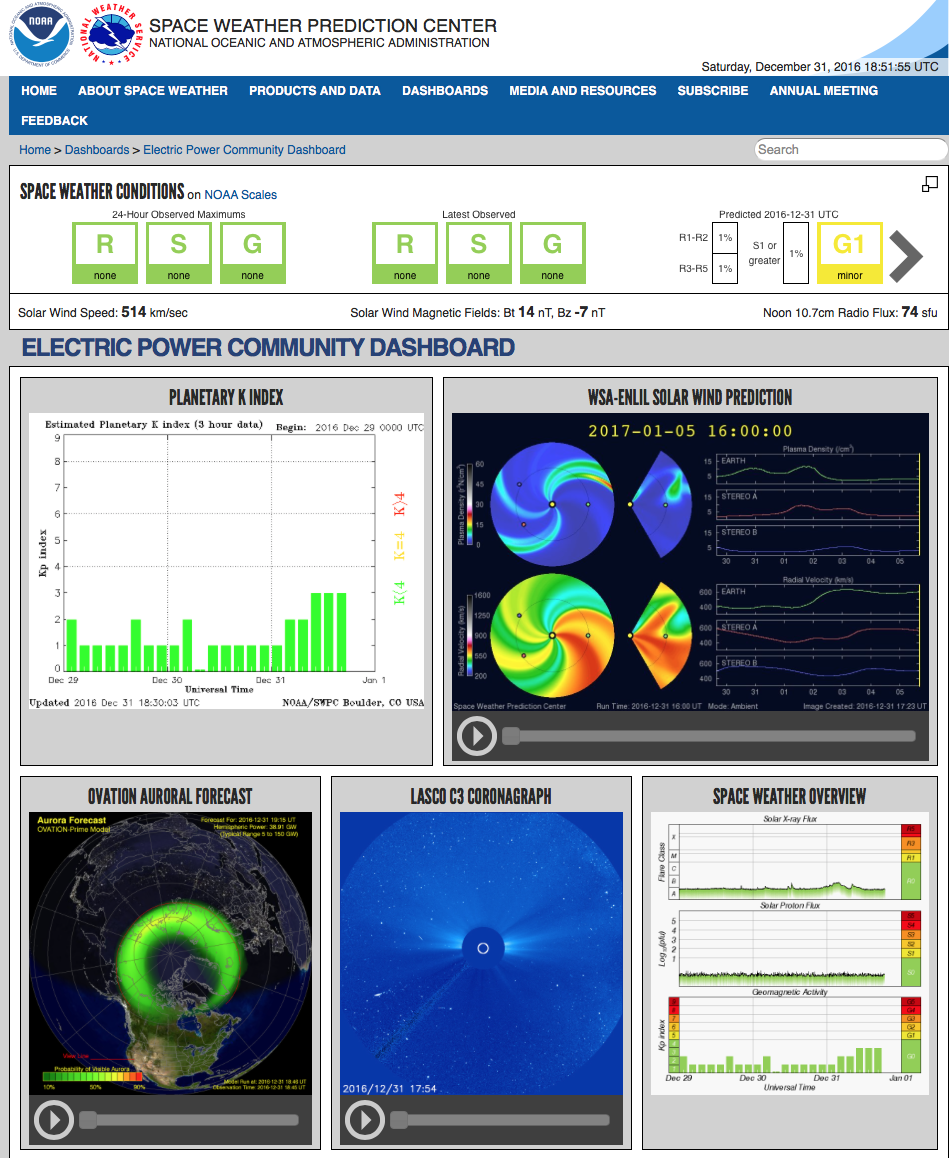
Today’s space weather forecast
Based on the Electric Power Community Dashboard from NOAA’s Space Weather Prediction Center, it looks like we have mild space weather on 31 December 2016. All three key indices are green: R (radio blackouts), S (solar radiation storms), and G (geomagnetic storms). That’s be a good way to start the New Year.
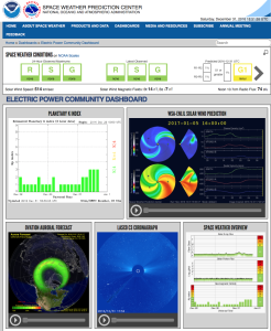
See your NOAA space weather forecast at:
http://www.swpc.noaa.gov/communities/electric-power-community-dashboard
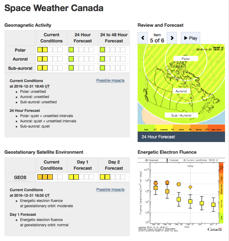
Natural Resources Canada also forecasts mild space weather for the far north.
 You can see the Canadian space weather forecast at the following link:
http://www.spaceweather.gc.ca/index-en.php
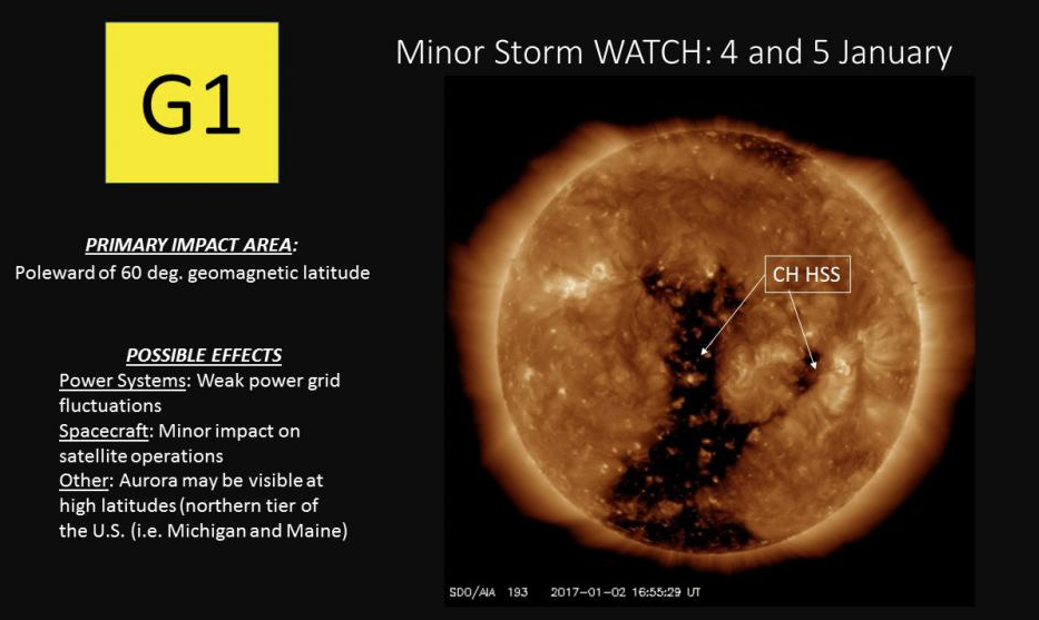
4 January 2017 Update: G1 Geomagnetic Storm Approaching Earth
On 2 January, 2017, NOAA’s Space Weather Prediction Center reported that NASA’s STEREO-A spacecraft encountered a 700 kilometer per second HSS that will be pointed at Earth in a couple of days.
“A G1 (Minor) geomagnetic storm watch is in effect for 4 and 5 January, 2017. A recurrent, polar connected, negative polarity coronal hole high-speed stream (CH HSS) is anticipated to rotate into an Earth-influential position by 4 January. Elevated solar wind speeds and a disturbed interplanetary magnetic field (IMF) are forecast due to the CH HSS. These conditions are likely to produce isolated periods of G1 storming beginning late on 4 January and continuing into 5 January. Continue to check our SWPC website for updated information and forecasts.”
The coronal hole is visible as the darker regions in the following image from NASA’s Solar Dynamics Observatory (SDO) satellite, which is in a geosynchronous orbit around Earth.
 Source: NOAA SWPC
SDO has been observing the Sun since 2010 with a set of three instruments:
- Helioseismic and Magnetic Imager (HMI)
- Extreme Ultraviolet Variability Experiment (EVE)
- Atmospheric Imaging Assembly (AIA)
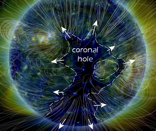
The above image of the coronal hole was made by SDO’s AIA. Another view, from the spaceweather.com website, provides a clearer depiction of the size and shape of the coronal hole creating the current G1 storm.
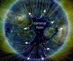 Source: spaceweather.com
You’ll find more information on the SDO satellite and mission on the NASA website at the following link:
https://sdo.gsfc.nasa.gov/mission/spacecraft.php
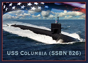 Columbia-class SSBN. Source: U.S. Navy
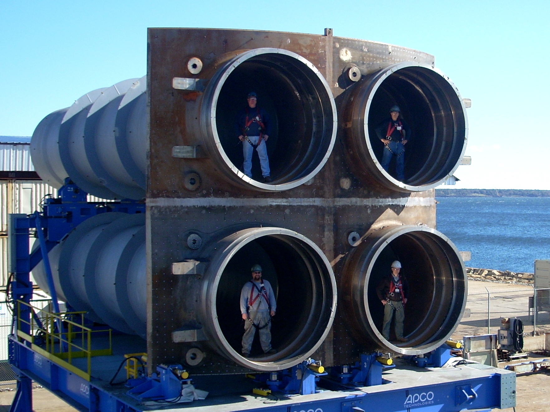 CMC “quad-pack.” Source: General Dynamics via U.S. Navy
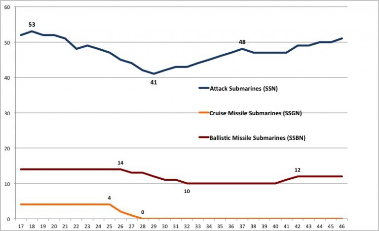 Source: U.S. Navy 30-year Submarine Shipbuilding Plan 2017


 Source: Taint