All posts by Drummer

Dividing by Zero

Peter Lobner

In 1967, the old Marchant electromechanical calculators in the physics lab were replaced by silent Wang electronic calculators.

The Marchant SCM Transflo Model TR shown below, manufactured after 1962, was a contemporary of the calculators replaced by the Wang.

Source: https://en.wikipedia.org/wiki/Marchant_calculator

The Wang 300-series electronic calculators were introduced in October of 1965, and the first machines went into production in March 1966.  The physics lab got a Wang system that looked like this.

Source: http://www.oldcalculatormuseum.com/wang360.html

This was the end of an era.  I could no longer vent my frustration at a calculation gone wrong by dividing by zero on several Marchant machines and leaving the room.

Why was this a problem for an electromechanical calculator?  These machines performed multiplication as a series of sequential additions and division were performed as a series of sequential subtractions.  The electromechanical Marchant calculator performed fully automatic division and would grind on until the final result was reached with a balance of zero in the “accumulator”, or until the last register on the machine had been filled and a small positive balance remained in the accumulator.

For example, 16 divided by 3 would be performed as:

16 -3 -3 -3 -3 -3 -3

At this point, the accumulator would be in “overdraft” (a negative value), the last subtraction would be cancelled by adding back +3, yielding a balance of +1 in the accumulator after 5 subtraction cycles. For a result set up for one decimal point accuracy, the calculation would continue as:

1 – 0.3 – 0.3 – 0.3 – 0.3

Again, the accumulator would be in “overdraft”, the last subtraction would be cancelled by adding back + 0.3, yielding a balance of + 0.1 in the accumulator after 3 subtraction cycles.

In this case, the result for 16 divided by 3 would be reported as 5.3.

Division by zero is the sequential subtraction of zero, over and over and over again. It’s an endless loop and the Marchant’s fully automatic division process was happy to oblige until someone got tired of the all the gear noise and cancelled the calculation (or pulled the plug).  These were durable machines.  I came into the lab one morning and found one Marchant still grinding away in an endless loop that probably started late the previous evening (I didn’t do it!).

Watch five old-school calculators grapple with division by zero here:

https://www.popularmechanics.com/technology/gadgets/g19695670/watch-five-old-school-calculators-grapple-with-division-by-zero/?src=nl&mag=pop&list=nl_pnl_news&date=040918

I guess you had to be there.

Thorium: What’s Old is New Again

Peter Lobner

Development of the uranium-thorium fuel cycle in the U.S began in the late 1940s, encouraged by the abundance of thorium, the ability to convert thorium into fissile uranium during reactor operation, and the prospects for a closed fuel cycle with good economics.  The commercial potential of thorium has yet to be realized.

Today, there is renewed interest in thorium as an abundant, cheap nuclear fuel source that can be employed in the context of a variety of proliferation-resistant nuclear fuel cycles.

1. In the beginning:

Alvin Weinberg is generally considered in the U.S. to be “father” of the pressurized water reactor (PWR), which has become the dominant type of nuclear reactor employed in commercial power generation and in naval reactors.  On 18 September 1944, Weinberg first described the basis for a PWR, with ordinary water as both coolant and moderator operating at high pressure, and producing steam for power production.

Dr. Alvin Weinberg. Source: Oak Ridge National Laboratory

On 10 April 1946, Weinberg and F. H. Murray (Oak Ridge, Clinton Laboratory) published, “High-Pressure Water as a Heat-Transfer Medium in Nuclear Power Plants,” in which the design characteristics of a water-cooled and moderated PWR were presented.  Interestingly, this PWR concept had a thorium-converter core, which used 233U as the fissile “seed” and thorium as the fertile “blanket” to breed more 233U during reactor operation.  This was similar in concept to the thorium-breeder core installed in the Shippingport commercial power reactor nearly 30 years later under the Department of Energy’s (DOE) Light Water Breeder Reactor (LWBR) Program.

The neutron absorption and decay chains for converting natural thorium (232Th) into fissile uranium (233U and 235U) are shown in the following diagram.

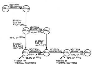
Source:  WAPD-TM-1387

Production of 233U through the neutron irradiation of 232Th invariably produces small amounts of 232U as an impurity (not shown in the above diagram), because of parasitic (n,2n) reactions on 233U itself, or on Pa233(protactinium), or on 232Th. The decay chain of 232U quickly yields strong gamma radiation emitters.  This characteristic is one aspect of the proliferation resistance of thorium fuel cycles.

2. Early commercial power reactors with thorium-converter cores

 In the U.S., thorium-converter cores were operated in five commercial power reactors between 1962 and 1989:

  • Indian Point 1 PWR
  • Elk River boiling water reactor (BWR)
  • Shippingport LWBR
  • Peach Bottom 1 high-temperature gas-cooled reactor (HTGR)
  • Fort St. Vrain HTGR

A brief overview of these commercial power reactors follows.  In retrospect, none would be judged as commercial successes.

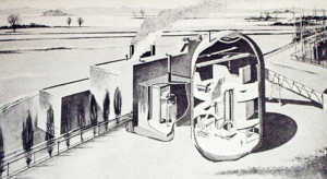
Indian Point 1 thorium-converter Core 1 (1962 – 1974)

The first commercial use of a thorium-converter “seed-and-blanket” core was in the Indian Point 1 pressurized water reactor designed by Babcock & Wilcox. Construction started in New York in May 1956 and the plant was commissioned in October 1962.

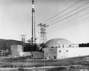
Indian Point 1, circa 1963. Source: USDOE, https://commons.wikimedia.org/

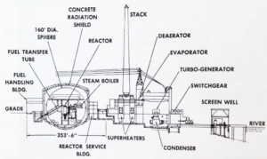
Indian Point 1 nuclear plant cross-section.   Source: Atomic Power Review, http://atomicpowerreview.blogspot.com/2013/02/carnival-145.html

Indian Point 1 was one of very few nuclear plants to incorporate fossil fired superheat to supplement the reactor power. In the cross-section view above, you can see the two oil-fired superheaters placed between the reactor and the turbine generator.  In its original configuration, Indian Point 1 had a net electrical output of 255 MWe, of which 104 MWe was derived from the fossil-fired superheaters.

Core 1 was rated at 585 MWt.  This was the only thorium converter core; highly-enriched (93%) 235U was used as the seed material. This core consisted of 120 fuel assemblies arranged in three concentric zones, each with differing UO2– ThO2ratios.  The central zone had the lowest uranium content.  Core loading was about 1,300 kg (2,425 pounds) of UO2(1,100 kg of U-235) and 17,207 kg (37,935 pounds) of ThO2.

The zoned core and fuel element layout are shown below.

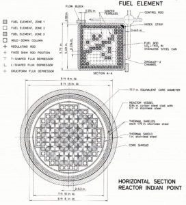
Source:  Directory of Nuclear Reactors, Volume IV, Power Reactors, International Atomic Energy Agency, 1962

Subsequent cores used low-enriched UO2fuel and were rated at a somewhat higher power, 615 MWt.  Core 2 was installed between the last quarter of 1965 and the first quarter of 1966, after three years of operation on the thorium-converter Core 1. With the all-UO2Core 2, the plant’s net electrical output was raised to 265 MWe.

Seventeen tons of stainless steel-clad thorium oxide pellet fuel from Core 1 were reprocessed at the privately owned and operated Nuclear Fuel Services plant at West Valley, New York.  This was the first commercial spent fuel reprocessing plant in the U.S.

The Indian Point 1 nuclear plant was shutdown in October 1974, after 12 years of operation.

Elk River thorium-converter core (1964 – 1968)

This small boiling water reactor (BWR) demonstration plant was developed by Allis-Chalmers and built in Minnesota. The reactor core, which was rated at 58.2 MWt, was a highly-enriched (93%) 235U / thorium converter.  Core loading was about 208 kg (459 pounds) of UO2and 4,300 kg (9,480 pounds) of ThO2in 148 fuel assemblies.

Like Indian Point 1, Elk River incorporated fossil fired superheat to supplement the reactor power.  The plant’s total thermal power was 73 MWt, yielding a net electrical output of 22 MWe. The general plant layout is shown below.

Source: http://atomicpowerreview.blogspot.com/2011/09/apr-atomic-journal-elk-river-1.html

The Elk River nuclear plant only operated from 1 July 1964 to 1 February 1968.  Subsequently, the plant was decommissioned. Some of the spent nuclear fuel was sent to the Trisaia facility in southern Italy for reprocessing as part of a thorium fuel cycle research program supported by the Italian National Committee for Nuclear Energy.  This pilot plant was operated during 1970s to process the uranium-thorium cycle fuels

Shippingport Light Water Breeder Reactor (LWBR, 1977 – 1982)

The LWBR Program, which was run for the Department of Energy (DOE) by the Office of Naval Reactors, was conducted to demonstrate the capability of the 233U/ thorium fuel system for use in a breeder reactor core that could be deployed in conventional light water reactor plants.  The LWBR core was installed in the Shippingport reactor and started operation in the fall of 1977.  Operation with the LWBR core finished on October 1, 1982.

Considerable experience was gained in fabricating the fuel for the LWBR core. This reactor used 233U / thorium instead of 235U / thorium as used in the Indian Point 1 and Elk River thorium converter cores.  The 233U needed for the LWBR was recovered from previously irradiated thorium using existing PUREX reprocessing equipment, which was designed for recovering uranium, but was not suitable for thorium recovery.  About 1,100 kg (2,425 pounds) of 233U was processed in pilot-plant scale equipment at Oak Ridge National Laboratory (ORNL) to produce the reactor-grade UO2needed for the LWBR core.  Fortunately, the 232U content of the uranium (note: 232U is a byproduct formed during thorium irradiation) was less than 10 ppm and remotely operated facilities with heavy shielding were not required to protect against high-energy gamma radiation from the 232U decay chain.

The basic LWBR seed-and-blanket core layout is shown in the following diagram:

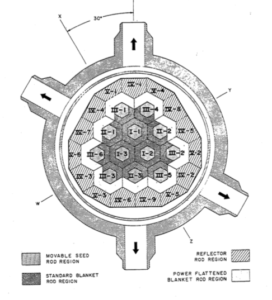
Source:  INEEL/EXT-98-00799, Rev. 1, “Fuel Summary Report: Shippingport Light Water Breeder Reactor,” January 1999

LWBR fuel modules consisted of a hexagonal seed module inside an annular blanket module. The movable seed modules started life below the blanket modules and traveled vertically upward through the hexagonal passages in the blanket modules during core life. Core reactivity was controlled by changing the axial position of seed modules within the surrounding blanket modules, thus eliminating parasitic loss of neutrons to conventional poison control rods.

In the March 1986 report, “Shippingport Operations With the Light Water Breeder Reactor Core,”WAPD-TM-1542, Bettis Atomic Power Laboratory reported the following results:

“The Shippingport Station during LWBR operation demonstrated flexibility and load change response characteristics superior to those found in non-nuclear steam generating stations and the availability of the LWBR reactor compared very favorably with conventional light water reactors. The core operated for five years accumulating 29,047 effective full power hours (EFPH), far beyond the design goal of 15,000 EFPH. At the end of this period, the core was removed and the spent fuel shipped to the Naval Reactors Expended Core Facility in Idaho for a detailed examination to verify core performance, including an evaluation of breeding characteristics.”

Westinghouse reported the breeding performance of the reactor as follows (WAPD-T-3007, October 1993):

“Nondestructive assay of 524 fuel rods and destructive analysis of 17 fuel rods determined that 1.39% more fissile fuel was present at the end of core life than at the beginning, thereby establishing that breeding had occurred. Successful LWBR power operation to over 160% of design lifetime demonstrated the performance capability of this fuel system.”

The LBWR spent fuel was not reprocessed.

High-temperature Gas-Cooled Reactors (HTGRs, 1967 – 1989)

Three U.S. HTGRs and two German HTGRs have operated with U-Th coated particle fuel.

  • Peach Bottom 1 (1967 – 1974)
    • 40 MWe General Atomics HTGR operated in Pennsylvania
    • Used highly-enriched 235U / thorium fuel in the form of microspheres of mixed thorium-uranium carbide coated with pyrolytic carbon. These microspheres were embedded in annular graphite segments that were arranged into fuel elements.
  • Fort St. Vrain (1976 – 1989)
    • 330 MWe General Atomics HTGR operated in Colorado
    • Used highly-enriched 235U / thorium fuel in the form of TRISO and BISO microspheres coated with pyrolytic carbon, which were embedded in a graphite matrix and placed in prismatic graphite fuel elements.  The TRISO fuel particles were highly-enriched 235U and the BISO fuel particles were thorium.
    • Almost 25 tonnes (25,000 kg, 55,155 pounds) of thorium was used in fuel for the reactor.
  • Thorium High Temperature Reactor (THTR, 1983 – 1989)
    • 300 MWe pebble-bed reactor operated in Germany.
  • AVR (1967 – 1988)
    • 15 MWe pebble-bed reactor operated in Germany.
    • AVR was the first reactor based on the circa 1945 – 46 concept of the “Daniels Pile” by Farrington Daniels, the inventor of pebble bed reactors.

In the U.S., General Atomics originally planned to have HTGR spent fuel reprocessed to recover useful material, including 233U, which would have been recycle in HTGR fuel. The planned back-end of the fuel cycle included a step to separate the TRISO and BISO particles, thereby simplifying the downstream reprocessing steps for uranium and thorium.

No commercial HTGRs were built in the U.S. after Fort St. Vrain and the back-end of the HTGR U-Th fuel-cycle was never developed.  Spent fuel from the operating U.S. HTGRs was not reprocessed. DOE took title to the spent fuel and became responsible for managing its temporary storage at the Fort St. Vrain site.

3. Reprocessing spent uranium – thorium fuel *

By the early 1950s, several kilograms of purified 233U had been recovered from experimental lots of irradiated thorium, and two chemical processing flowsheets based on solvent extraction techniques had been developed and tested in small-scale operations.

The THOREX process was developed in the mid-1950s for reprocessing 233U – thorium fuel.  By the mid-to-late 1950s, the THOREX Pilot Plant Demonstration Program had been completed, and 35 tons of irradiated thorium metal had been processed in a facility with a throughput of 150 to 200 kg of thorium per day to recover 55 kg of purified 233U. The principal emphasis was on demonstrating the THOREX flowsheet, defining flowsheet capabilities, and identifying problem areas in the reprocessing of spent U-Th fuel.

During the 1960s, approximately 870 tons of thorium (primarily as ThO2) was irradiated. This thorium was then processed in production scale equipment to recover 1.4 tons of purified233U. The large-scale programs at Savannah River Plant (SRP) and Hanford utilized either the THOREX Flowsheet or a modified version of it (i.e., the Acid THOREX flowsheet) to effect the separation and recovery of 233U and thorium.

In the late 1970s, a total of 28 metric tons of fabrication scrap generated during the preparation of LWBR fuel was recycled in large-scale solvent extraction facilities to recover the 233U. The ability to dissolve advanced ThO2-containing fuels was an important step in demonstrating the reprocessing of spent fuel in a U-Th fuel cycle.

The DOE HTGR Fuel Recycle Program supported research and development for reprocessing HTGR fuel, focusing on small, engineering-scale tests.  No pilot- or full-scale reprocessing facility was built.

In April 1977, President Carter terminated federal support for reprocessing in an attempt to limit the proliferation of nuclear weapons material. The U.S. nuclear fuel cycle became the once-through fuel cycle we have today.

*          Source: “THOREX Reprocessing Characterization,” International Nuclear Fuel Cycle Evaluation (INFCE), 1978

4. The Radkowsky Thorium Reactor (RTR) concept

 Alvin Radkowsky, who was recruited by Admiral Rickover in 1947, later served as the Chief Scientist of the Naval Reactors program. He was responsible for originating and assisting in the development of two reactor concepts for which he was awarded the Navy’s Distinguished Civilian Award (the highest non-military award) in 1954 and the Atomic Energy Commission (AEC) Citation (1963):

  • Burnable poison, which is important to all nuclear power plants for managing long-term reactivity control, and is especially important for enabling very long life naval reactor cores.
  • Seed and blanket reactor core, which consists of a highly enriched fuel “seed” section surrounded by a “blanket” of fertile natural uranium. The blanket generates more than half of the reactor power and has a very long life relative to the “seed” section, which is replaced more frequently.

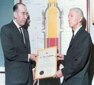
Alvin Radkowsky receives award from Admiral Hyman Rickover.  A diagram of the Shippingport reactor with a seed-and-blanket core is in the background. Source:  Thorium Power, Inc.

With the encouragement of Edward Teller, Alvin Radkowsky developed a long-standing interest in the use of thorium in nuclear reactors as a means to improve resistance to the proliferation of nuclear material suitable for making weapons. He held several patents in the field, which he assigned to the company he helped found in 1992, Thorium Power, Inc.

The Radkowsky Thorium Reactor concept developed by Alvin Radkowsky and Thorium Power makes use of a seed-and-blanket geometry with low-enriched (< 20%) 235U as the initial fissile seed material and thorium as the fertile blanket material.  Unlike Indian Point 1 and the LWBR, which separated the seed and blanket elements into zones in the core, the RTR implements the seed-and-blanket concept at the level of individual fuel assemblies that are designed to replace the fuel assemblies in existing reactors, but require a complex process to manage fuel during refueling outages. Radkowsky described his RTR fuel design concept as follows:

“Basically, seeds are treated similarly to the standard PWR assemblies. i.e., approximately one-third of seeds are replaced annually by “fresh” seeds, and the remaining two-thirds (partially depleted) seeds are reshuffled. Each seed is loaded into an “empty” blanket, forming a new fuel type. These new fuel type (fresh) assemblies are reshuffled together with partially depleted SBU (seed-blanket) assemblies to form a reload configuration for the next cycle.……..the Th-blanket in-core residence time is quite long (about 10 years), while the uranium part of the SBU (seed) is replaced on a annual (or 18 month) basis, similar to standard PWR fuel management practice.”

You can read his paper entitled, “Thorium Fuel for Light Water Reactors – Reducing Proliferation Potential of Nuclear Power Fuel Cycle,”here:

http://www.iaea.org/inis/collection/NCLCollectionStore/_Public/28/023/28023771.pdf

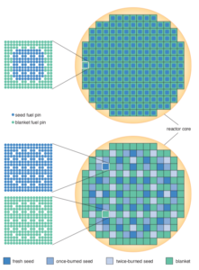
The RTR seed-and-blanket fuel assembly concept and the simpler zoned seed-and-blanket core concept are well illustrated in the following figure from an article by Mujid S. Kazimi entitled, “Thorium Fuel for Nuclear Energy.”  The RTR core and the seed-and-blanket arrangement of the fuel rods in an individual fuel assembly are shown at the top of the diagram.  A more conventional seed-and-blanket core with separate seed and blanket assemblies is shown at the bottom of the diagram.

You can read Mujid Kazimi’s complete article on the American Scientist website here:

https://www.americanscientist.org/sites/americanscientist.org/files/200582141548_306.pdf

The September / October 1997 issue of the The Bulletin of the Atomic Scientists contains an article by John S. Friedman entitled, “More power to thorium?” in which the author offered the following comments on the RTR:

“The Radkowsky design avoids recycling by envisioning a complex fuel core in which uranium “seeds” enriched to about 20 percent uranium 235 are kept separate from a surrounding thorium-uranium “blanket.” The uranium 235 produces the neutrons that sustain the chain reaction while slowly creating uranium 233 in the blanket. As burnup continues, the newly created uranium 233 picks up an increasingly greater share of the fission load.”

“As in any uranium-fuel reactor, the uranium portion of the core would produce plutonium, but in lesser quantities than in a conventional reactor and with far higher isotopic contamination (from Pu-238, which is a strong alpha radiation emitter). The latter characteristic would make the plutonium even less desirable for weapons than is ordinary reactor-grade plutonium, argues Radkowsky. That would make his reactor exceptionally unattractive to would-be weapons makers. Although uranium 233 can be used for weapons, it too would be isotopically contaminated (from U-232, which is a strong, high-energy gamma radiation emitter), making its use in weapons unlikely.”

“The main selling point of the Radkowsky concept, according to Grae, is that the reactor ‘helps sever the link between nuclear power generation and nuclear weapons.’ The new reactor, he says, will help fulfill the mandate of the Nuclear Non-Proliferation Treaty, which calls not only for a halt in the proliferation of nuclear weapons, but also for the transfer of peaceful nuclear technology.”

You can read John Friedman’s complete article here:

https://ltbridge.com/wp-content/uploads/2017/08/19.pdf

Thorium Power, Inc. has worked with Kurchatov Institute, Brookhaven National Laboratory and others to design and analyze the use of hexagonal RTR-type thorium-plutonium fuel assemblies that could replace the standard fuel assemblies in Russian-designed VVER-1000 PWRs.  Analysis in 2001 indicated that large quantities of weapons-grade plutonium could be consumed over the 40 year operating life of a VVER-1000 reactor.

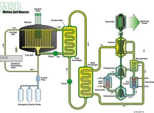
5. Molten salt thorium reactors

Molten salt reactors (MSRs) use molten fluoride salts as the primary coolant.  The main MSR concept is to have the fuel dissolved in the coolant as a fuel salt that is continuously circulated through the primary system and into a “reactor vessel” where a controlled criticality is maintained to produce useful power. The system operates at high temperature and low pressure.  The MSR concept could include provisions for on-line cleanup and reprocessing of the circulating fuel salt.

In the U.S., the DOE conducted an MSR program from 1957 to 1976. The small 8 MWt test reactor known as Molten Salt Reactor Experiment (MSRE) ran two campaigns at ORNL; the first campaign (1965 – 68) ran with 235U and the second campaign (1968 – 1969) ran with imported (not bred) 233U.  Thorium was not used in MSRE.

MSRE demonstrated the feasibility of the MSR concept and provided the technical basis for designing an MSR breeder using thorium with a graphite moderator in a core operating on thermal neutrons.  The MSR breeder never got past the study phase.

The Generation IV (Gen IV) International Forum, which was initiated by the U.S. Department of Energy in 2000, has been promoting a fast-spectrum molten salt reactor (MSFR) with dissolved 233U and thorium fuel. The Gen IV MSR power system concept is shown in the following diagram.  Construction and operation of any Gen IV reactor concept is decades away.

Source:  Gen IV International Forum.  https://www.gen-4.org/gif/jcms/c_42150/molten-salt-reactor-msr

In August 2017, the Salt Irradiation Experiment (SALIENT) began operation at the Petten High Flux Reactor in the Netherlands.  This is the first in-reactor experiment with molten salt in about 40 years. SALIENT will conduct tests on thorium molten salt in an actual reactor environment. The results of the SALIENT tests are intended to support future development of a European MSR thorium breeder reactor. You can read the Petten announcement here:

https://articles.thmsr.nl/petten-has-started-world-s-first-thorium-msr-specific-irradiation-experiments-in-45-years-ff8351fce5d2

6. India’s thorium fuel plan

 India is the only country in the world that has established a fully committed thorium program.  Because India is outside the Treaty on the Non-Proliferation of Nuclear Weapons (NPT) due to its nuclear weapons program, it was for 34 years largely excluded from trade in nuclear plants and materials, which hampered its development of civil nuclear energy. Due to this trade ban and lack of indigenous uranium, India has been developing a unique nuclear fuel cycle to exploit its reserves of thorium. India has the second largest known reserve of thorium in the world (Australia is #1). In September 2008, the international Nuclear Suppliers Group (NSG) issued a waiver, which allowed India to commence international nuclear trade.  This has secured access to a uranium supply chain and opened the Indian nuclear market to various LWR commercial power plants from international suppliers.

India has developed a three-stage thorium fuel plan that involves three types of reactors and a closed nuclear fuel cycle.

  • Stage 1: Deployment of indigenous pressurized heavy-water reactors (PHWRs) to produce plutonium.
    • The PHWR designed by Bhabha Atomic Research Centre (BARC) is a horizontal pressure tube / calandria reactor using natural uranium dioxide (UO2) fuel and heavy water as moderator and coolant.
    • India currently operates 18 PHWRs power plants, with generating capacities between 100 to 540 MWe.
    • Four 700 MWe PHWRs are under construction.
    • At least 16 more 700 MWe PHWRs are planned.
    • In the mid-1990s, India began using thorium in fuel assemblies in PHWR initial cores to even out the core power distribution (flux flattening) to allow the reactor to operate at full power in its initial phase of operation.

You’ll find a detailed description of India’s PHWR here:

https://www.iaea.org/NuclearPower/Downloads/Technology/meetings/2011-Jul-4-8-ANRT-WS/2_INDIA_PHWR_NPCIL_Muktibodh.pdf

  • Stage 2: Deployment of indigenous fast-neutron reactors with blankets containing uranium and thorium to breed new fissile material (Pu and 233U).
    • The Prototype Fast Breeder Reactor (PFBR) designed by the Indira Gandhi Centre for Atomic Research is a sodium-cooled pool-type reactor rated at 500 MWe.
    • The PFBR initially will be fueled with a plutonium-uranium mixed oxide (PuO2– UO2) fuel.
    • PFBR is nearing completion at the Madras Atomic Power Station in Kalpakkam. Commissioning is expected in early-to-mid 2018 and commercial power generation may occur by end of 2018.
    • The Indian government in 2013 approved construction at Kalpakkam of fuel cycle facilities to recover plutonium and uranium, to be ready in time to process the first used fuel from the PFBR.
    • After PFBR, India plans to build six larger fast breeder reactors rated at 600 MWe.

You’ll find a description of the PFBR and the fast reactor fuel cycle at the following links:

http://fissilematerials.org/library/igcar03.pdf

and,

http://www.theenergycollective.com/dan-yurman/2410617/india-commits-fast-reactor-fuel-cycle-facility-u-233

  • Stage 3: Deployment of advanced heavy-water reactors (AHWR) designed by BARC to demonstrate commercial utilization of thorium.
    • The AHWR is a 300 MWe, vertical pressure tube type, boiling light water cooled, heavy water moderated reactor.
    • The fuel material will use Th-Pu MOX and Th-U MOX, where the uranium may be 233U or LEU 235U.  Development of Th-Pu and 233U-Th MOX fuels was initiated in 2001.
    • The reactor is configured to obtain a significant portion of power by fission of 233U derived from in-situ conversion from 232Th. On an average, about 39% of the power will be obtained from thorium.
    • One AHWR prototype currently is planned.  Start of construction has been delayed several times since it was first announced in 2004.  Start of construction in 2018 is possible.
    • BARC claims that the AHWR will have a one hundred year design life.

You’ll find more information on the AHWR at the following links:

http://www.barc.gov.in/reactor/ahwr.pdf

and,

https://aris.iaea.org/PDF/AHWR.pdf

7. Summary

So, there you have it.  Early experience with thorium fuel provided a technical proof-of-concept demonstration of thorium fueled reactors, but was not a commercial success.  A complete closed fuel cycle with thorium has never been demonstrated.

The key factor driving the resurgence of international interest in thorium is the proliferation resistance of the Th-U and Th-Pu fuel cycles.  The key factors driving India’s interest in thorium are the abundance of thorium and shortage of uranium in that nation coupled with India’s three-stage thorium fuel plan, which was developed to counter its long-term isolation from international trade in nuclear plants and materials as a consequence of not signing the NPT.

Work in Russia on Radkowsky Thorium Reactor (RTR) fuel elements and renewed work on a thorium molten salt reactor (MSR) in Europe certainly are encouraging.  However, there’s a long road (decades) from where these projects stand today and actual thorium utilization in a commercial nuclear power plant.  The most promising near-term (within a decade) demonstration of commercial utilization of thorium will be India’s AHWR and the associated thorium closed fuel cycle.

Additional resources on thorium:

“Nuclear Power in India”, World Nuclear Association:  http://www.world-nuclear.org/information-library/country-profiles/countries-g-n/india.aspx

CHEUK WAH LAU, “Improved PWR Core Characteristics with Thorium-containing Fuel”, Thesis for the Degree of Doctor of Philosophy, 2014:  https://www.kth.se/polopoly_fs/1.597223!/Improved%20PWR_Cheuk%20Wah%20Lau.pdf

Michael J. Higatsberger, “The Non-Proliferative Commercial Radkowsky Thorium Fuel Concept,”November 1999:  https://ltbridge.com/wp-content/uploads/2017/08/16.pdf

Gravitational Waves Come in Colors

Peter Lobner

On 14 September 2015, the Laser Interferometer Gravitational-Wave Observatory (LIGO) ushered in a new era in astronomy and astrophysics by opening a part of the gravitational wave spectrum to direct observation. In my 17 February 2017 post,“Perspective on the Detection of Gravitational Waves,” I included the following graphic from an interview of Kip Thorne by Walter Issacson.

Source: screenshot from Kip Thorne / Walter Issacson interview at: https://www.youtube.com/watch?v=mDFF27Nr-EU

The key point of this graphic is to illustrate how the LIGO detector is able to “see” only a part of the gravitational wave spectrum.  The LIGO team reported that the Advanced LIGO detector is optimized for “a range of frequencies from 30 Hz to several kHz, which covers the frequencies of gravitational waves emitted during the late inspiral, merger, and ringdown of stellar-mass binary black holes.”  This is the type of event associated with the first several gravitational wave detections. The European Advanced VIRGO detector, which came on line in 2017, operates on the same principle as LIGO, precisely measuring differences in the times-of-flight of laser beams in the two legs of a long baseline interferometer. VIRGO is optimized to view a range of gravitational wave frequencies from about 10 Hz to 10 kHz.

On 17 August 2017, LIGO and VIRGO detected gravitational waves from a different source: the collision of two neutron stars. Unlike the previous gravitational wave detections from black hole coalescence, the neutron star collision that produced GW180817 also produced other observable phenomena in multiple wavelength bands. LIGO and VIRGO triangulated the source of this gravitational wave event, which also was observed by dozens of telescopes on the ground and in space, as shown in the following diagram.

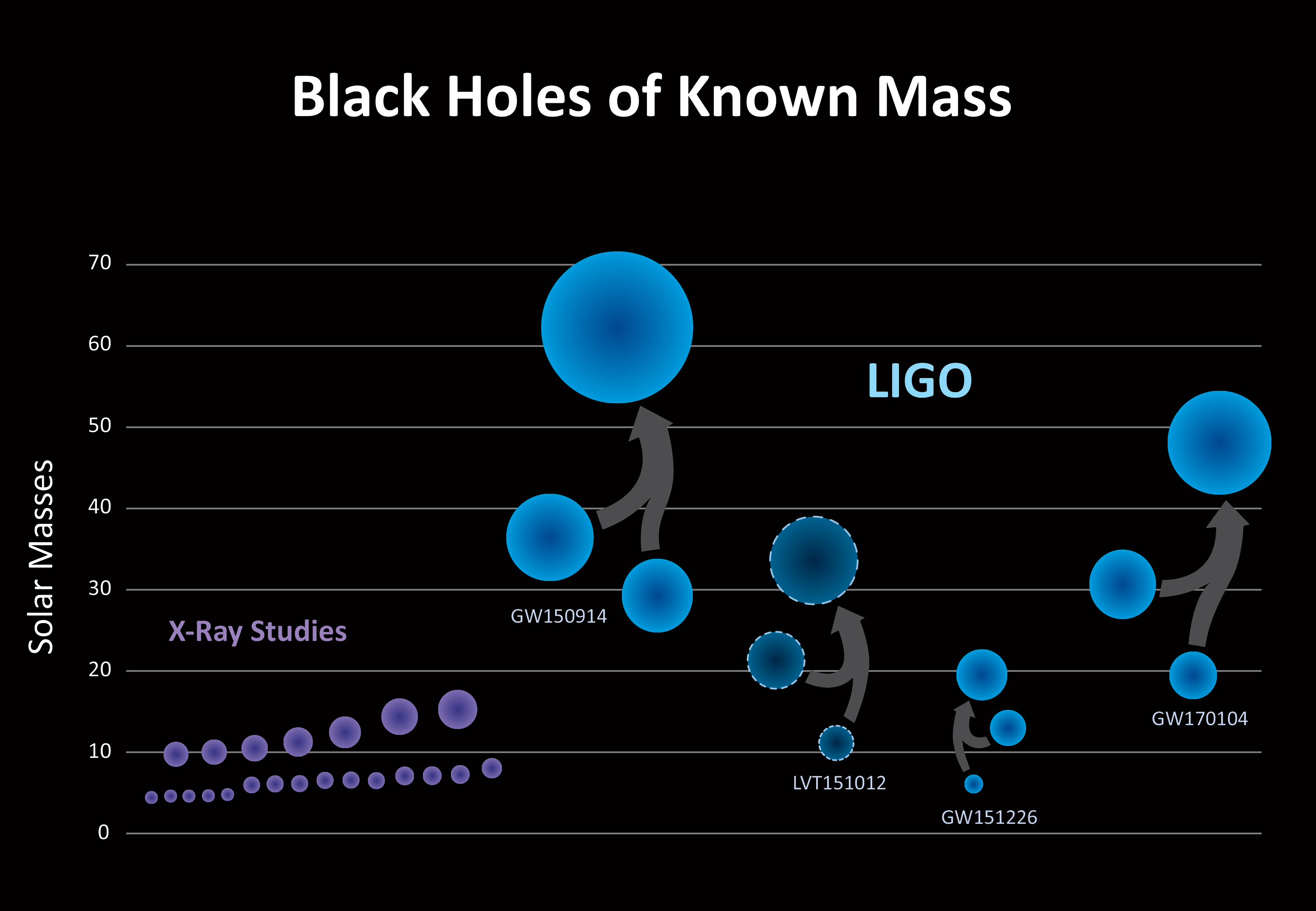
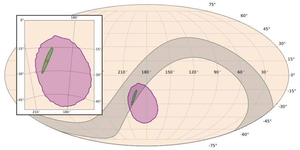
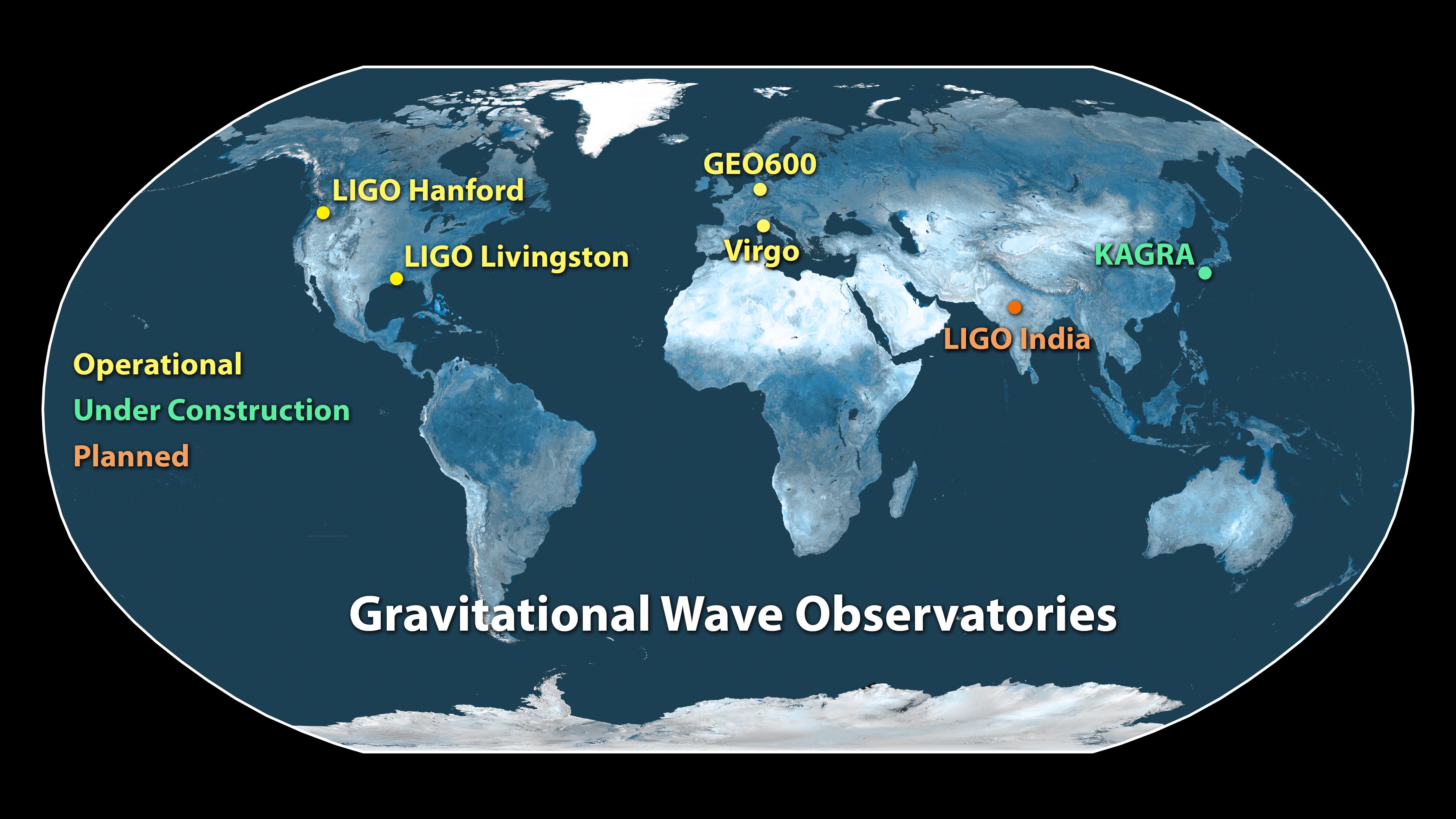
Source: LIGO – VIRGO, https://www.ligo.org/detections/GW170817/images-GW170817/GW+EM_Observatories.jpg

The ability to cue a worldwide array of multi-spectral observatories on short notice greatly added to the depth of understanding of the GW170817 event.  The international collaboration on this event was a great example of the benefits of “multi-messenger” astronomy. For more information, see my 25 October 2017 post, “Linking Gravitational Wave Detection to the Rest of the Observable Spectrum.”

At the 11 April 2018 Lyncean Group meeting, Dr. Rana Adhikari, Professor of Physics, Mathematics and Astronomy at Caltech, provided an update on LIGO in his presentation, “The Dirty Details of Detecting Gravitational Waves from Black Holes.” You can view Dr. Adhikari’s presentation slides at the following link:

https://lynceans.org/talk-119-4-11-18/

As we have seen, the LIGO class of gravitational wave detector is capable of seeing large amplitude, relatively high frequency gravitational waves from very powerful, discrete events: stellar-mass binary black hole coalescence and neutron star collisions.

As shown in the above graphic, viewing lower frequency (longer wavelength) gravitational waves requires different types of detectors, which are discussed below.

LISA –  Laser Interferometer Space Antenna

This will be a very long baseline, equilateral triangular laser interferometer in space, established of three spacecraft flying in formation in an Earth-trailing heliocentric orbit.  Each leg of the space interferometer will measure 2.5 million kilometers (1.55 million miles), about 625,000 times the length of the LIGO baseline (4 km, 2.49 miles). Each spacecraft will contain a gravitational wave detector sensitive at frequencies from about 10-4 Hz to 10-1 Hz, well below the frequency range of LIGO and VIRGO.

The European Space Agency’s (ESA) LISA Pathfinder spacecraft, which was launched in 2015 and ended its mission in July 2017, validated the technology for the LISA space interferometer.

Source: ESA, https://www.elisascience.org/

ESA reported:

“Analysis of the LISA Pathfinder mission results towards the end of the mission (red line) compared with the first results published shortly after the spacecraft began science operations (blue line). The initial requirements (top, wedge-shaped area) and that of the future gravitational-wave observatory LISA (middle, striped area) are included for comparison, and show that LISA Pathfinder far exceeded expectations.”

The ESA is planning to launch LISA in the 2029 – 2032 timeframe.  See my 27 September 2016 post, “Space-based Gravity Wave Detection System to be Deployed by ESA,” for additional information on LISA.  The LISA mission website is at the following link:

https://www.elisascience.org

PTA – Pulsar Timing Array

A pulsar is a highly magnetized rotating neutron star or white dwarf that emits a beam of electromagnetic radiation. This radiation can be observed only when the beam is pointing toward Earth.

PTA gravitational wave detection is based on correlated radio-telescope observations of an array of many pulsars known as “millisecond pulsars” (MSPs).  The signal from an MSP has a very predictable time-of-arrival (TOA), thereby allowing each MSP to function as a galactic “clock.”  Small disturbances in each “clock” are measurable with high precision on Earth.  In essence, the distance between an MSP and the observing radio-telescope forms one leg of a gravitational wave detector, with the leg length being measured in light-years.  A disturbance from a passing gravitational wave would to have a measurable signature across the many MSPs in the pulsar timing array.

A PTA is intended to observe in a different range in gravitational wave frequencies than LIGO and VIRGO, and is expected to see a different category of gravitational wave sources. Whereas LIGO and VIRGO can detect gravitational waves in the tens to thousands of Hz (audio) range, radio-telescope observatories currently are using PTAs to search for gravitational waves in the tens to hundreds of microHertz (10-6Hz) range with prospects of getting down to the 10-8Hz range. The primary source of gravitational waves in this frequency range is expected to be super-massive black hole binaries (billions of solar masses), which are believed to exist throughout the universe at the center of galaxies.

The International Pulsar Timing Array (IPTA) is an international collaboration among the following radio-telescope consortia: European Pulsar Timing Array (EPTA), the North American Nanohertz Observatory for Gravitational Waves (NANOGrav), and the Parkes Pulsar Timing Array (PPTA).  The goal of the IPTA is to detect gravitational waves using an array of about 30 MSPs. IPTA reports:

“Using telescopes located around the world is important, because any single telescope can see (a particular) pulsar … for much less than twelve hours, depending on the observing site’s latitude. Thus, the telescopes “trade off” between one another – as the pulsar sets from the perspective of, say, the Parkes telescope in Australia, it rises from the perspective of the Lovell telescope in the UK.”

You’ll find more information on IPTA on their website at the following link:

http://www.ipta4gw.org

You can visit the NANOGrav website here:

http://nanograv.org

Continuous gravitational waves

On 10 April 2018, the Max Planck Institute for Gravitational Physics announced the formation of a permanent Max Planck Independent Research Group under the leadership of Dr. M. Alessandra Papa to search for continuous gravitational waves.  The primary goal of this research group is to make the first direct detection of gravitational waves from rapidly rotating neutron stars. You can read this announcement here:

http://www.aei.mpg.de/2236875/searchingcontinuouswaves

Generation of the weak, continuous gravitational waves depends on the neutron star having an asymmetry that would perturb the stars gravitational field as it rapidly rotates. The method for detecting these weak, continuous gravitational waves was not described in the Planck Institute announcement.

CMB – Cosmic microwave background

The CBM is believed to be an artifact of the Big Bang and could carry evidence of the primordial gravitational waves from that era.  Such evidence would be expected to stretch across broad areas of the observable universe.

The European Space Agency (ESA) developed the Planck space observatory to map the CMB in microwave and infrared frequencies at unprecedented levels of detail. The Planck spacecraft was launched on 14 May 2009 and operated until 23 October 2013.  In 2016, the ESA released the results of the Planck all-sky survey of the CBM, which revealed that the universe appears to be isotropic, at least at the resolution of the Planck space observatory.  Researchers found that the actual CMB shows only random noise and no signs of patterns.

Planck all-sky survey. Source; ESA / Planck Collaboration

You’ll find more information on the Planck mission in my 28 September 2016 post, “The Universe is Isotropic.”

You can access ESA’s Planck science team home page here:

https://www.cosmos.esa.int/web/planck/home

In summary

The North American Nanohertz Observatory for Gravitational Waves (NANOGrav) website contains the following summary chart, which is an alternate view of the chart at the start of this article (from the Kip Thorne / Walter Issacson interview).  The NANOGrav chart provides a good perspective on the observational technologies that are opening windows into the broad spectrum of gravitational waves and their varied sources.

So, in an analogy to the optical spectrum and the range of colors we see every day, the primordial gravitational waves in the CBM would be at the “red” end of the gravitational wave spectrum. The much higher frequency gravitational waves seen by LIGO and VIRGO, from stellar-mass binary black hole coalescence and neutron star collisions, would be at the “violet” end of the gravitational wave spectrum. The LISA space-based interferometer will be looking in the “blue-green” range, while PTA observatories are looking in the “yellow-orange” range.

For more information on the current state of gravitational wave technology, you’ll find a good survey article by Davide Castelvecchia, entitled “Here Come the Waves,” in the 12 April 2018 issue of Nature, which you can read here:

https://www.nature.com/magazine-assets/d41586-018-04157-6/d41586-018-04157-6.pdf

1962 Nuclear Test in the Pacific Near San Diego

Peter Lobner

Everyone has heard about the atmospheric and underground nuclear tests that were conducted at the Nevada Test Site (NTS) from 1951 to 1992. NTS, which is about 394 miles (634 km) north of San Diego, CA, was the site of 928 nuclear tests.

Operation Dominic, was a series of 31 atmospheric or underwater nuclear tests conducted by the U.S. from April to October 1962 after the Soviet Union resumed atmospheric testing. One of the Operation Dominic tests occurred near San Diego, in the waters of the Pacific Ocean 426 miles (685 km) west of San Diego, CA at latitude 31° 14.7 N and longitude 124° 12.7’ W. This was U.S. nuclear test #238, code named Swordfish.

Swordfish test site west of San Diego, CA. Source: Google maps

Swordfish was a live-fire test of a nuclear-armed RUR-5A ASROC (Anti-Submarine ROCket) that was armed with a W44 nuclear warhead with a yield estimated to be about 10 kilotons (kT).

Mark 12 eight-cell ASROC launcher. Source: U.S. Navy / Wikipedia

ASROC launch. Source: seaforces.org

This was an operational test of the ASROC weapons system and a weapons effects test. The test would validate the nuclear-armed ASROC, which was being widely deployed in the fleet. In addition, the test would help define the effects of the nuclear detonation on the target and on nearby elements of an anti-submarine surface attack unit. The weapons effects data were needed to help the Navy establish a tactical doctrine for ASROC warhead delivery. The test sought to clarify tactical matters such as:

  • Minimum delivery range (safe standoff distance), with varying degrees of damage to the launching ship
  • Restrictions due to radioactivity on subsequent ship maneuvers Degree to which data from the Navy’s traditional high-explosive shock tests of ships applied to nuclear explosions
  • Safe standoff distance for delivery of nuclear weapons from submarines

The test also sought to determine:

  • Impact of the detonation on the U.S. strategic hydro-acoustic detection system known as SOSUS (SOund SUrveillance System)
  • Validation of models for detecting and classifying underwater nuclear explosions
  • Long-term drift and diffusion of radioactive contamination in the ocean environment.

The test was conducted on 11 May 1962 by Joint Task Group 8.9, which was led by aircraft carrier USS Yorktown (CV-10), was comprised of 19 ships, two submarine and 55 naval aircraft. JTG 8.9 included three Gearing-class destroyers, the submarine USS Razorback (SS-394) and landing ship dock USS Monticello (LSD-35).

  • Monticello set the instrumentation array for the test,
  • One destroyer (Bausell) was positioned about one mile the blast to monitor surface effects and the crew was evacuated
  • The Razorback monitored underwater effects from a distance of about 2.5 miles.

The nuclear-armed ASROC was fired from the destroyer USS Agerholm (DD-826) at a target 2.5 miles (4,348 yards / 4 km) away.  After the booster rocket burned out, the W44 nuclear depth charge warhead separated and flew a ballistic trajectory to the target. After impacting the water, the warhead sank to a prescribed depth, believed to be about 650 feet (198 meters) for the Swordfish test, before detonating.

USS Agerholm in the foreground of the Swordfish test. Source: Navsource.org

View from a helicopter trailing the USS Yorktown, 9,850 yards (3 km) from the Swordfish test. Source: Federation of American Scientists, fas.org

You can watch a short video clip of the Swordfish test from the perspective of the helicopter trailing USS Yorktown here:

https://gfycat.com/FlimsyTallEland

You can watch a longer video on the Swordfish test at the following link:

https://www.youtube.com/watch?v=EV5q_mlhaiM

You can read Test Director W.W. Murray’s detailed report, “Operation Dominic, Shot Swordfish, Scientific Director’s Summary Report,” dated 21 January 1963, here:

https://www.scribd.com/document/292806204/Swordfish-1962-Underwater-ASROC-Nuclear-Weapon-Test-Effects-Report

Some key points reported by the Test Director were:

  • The water above “surface zero” was left radioactively contaminated after the collapse of the plumes (and the base surge from the detonation).
  • For about an hour after an ASROC burst, the contaminated water left about surface zero will pose a radiological hazard of significance, even under the exigencies of a wartime situation.
  • Swordfish re-emphasized the role of the base surge as a carrier of radioactivity. A ship which maneuvers, following an ASROC burst, so as to remain at least 350 yards (320 meters) from the edge of the base surge will not subject its personnel to radiation doses in excess of peacetime test limits.
  • The contaminated water pool produced by an ASROC burst drifts with the current while it diffuses and decays radioactively.
  • After Swordfish, the pool was tracked for more than 20 days; in 20 days after the burst the center had drifted about 50 miles (80.5 km) south of surface zero and maximum surface radiation intensity measured 0.04 mr/hr.

A shorter summary on the Swordfish test is included Defense Nuclear Agency report DNA-6040F, “Operation Dominic – 1962,” (see p. 196 – 204), which you can read and download here.

http://www.dtic.mil/dtic/tr/fulltext/u2/a136820.pdf

All ASROC nuclear warheads were removed from service in 1989.

You’ll find a complete listing of all U.S. nuclear tests in the Department of Energy’s December 2000 report, “United States Nuclear Tests July 1945 Through September 1992,” (DOE/NV—209-REV 15), which you can read and download here.

https://web.archive.org/web/20061012160826/http://www.nv.doe.gov/library/publications/historical/DOENV_209_REV15.pdf

Integrity in Research

Peter Lobner

It’s hard to believe that this matter has become a significant issue in modern scientific research, but I’m sure that we’ve all read about questionable research practices, false claims in research papers, retraction of some papers, and notable researchers being exposed for their lack of scientific integrity. It appears that political bias and pressure  play roles in challenging integrity in some research.

The National Academies has just published a consensus study report entitled (you guessed it), “Fostering Integrity in Research.”

         Source: NAP

In their abstract, the National Academies authors explain:

“The integrity of knowledge that emerges from research is based on individual and collective adherence to core values of objectivity, honesty, openness, fairness, accountability, and stewardship. Integrity in science means that the organizations in which research is conducted encourage those involved to exemplify these values in every step of the research process. Understanding the dynamics that support – or distort – practices that uphold the integrity of research by all participants ensures that the research enterprise advances knowledge.”

If you have a MyNAP account (it’s free), you can download a pdf copy of this report for free from the National Academies Press (NAP) website at the following link:

https://www.nap.edu/catalog/21896/fostering-integrity-in-research

This report is a follow-on to a related two-volume, 1992 National Academies report entitled, “Responsible Science: Ensuring the Integrity of the Research Process,” which you can download here:

Volume 1:

https://www.nap.edu/catalog/1864/responsible-science-volume-i-ensuring-the-integrity-of-the-research

Volume 2:

https://www.nap.edu/catalog/2091/responsible-science-volume-ii-background-papers-and-resource-documents

In our world where “fake news” is becoming commonplace, responsible researchers must maintain their scientific integrity as they face various pressures to do otherwise.

Update 9 June 2019:  RAND Corporation issues a report on ethics in scientific research

In January 2019, RAND Corporation posted research report RR2912, “Ethics in Scientific Research – An Examination of Ethical Principles and Emerging Topics,” on the RAND website.

    Source: RAND Corporation, 2019

In their report abstract, RAND reported:

“The authors reviewed literature from across scientific disciplines and conducted interviews with experts in the United States, Europe, and China. The research had two motivations: (1) to inform researchers and sponsors who engage in research in emerging scientific disciplines and who may face new ethical challenges, and (2) to inform research sponsors — including government officials — who wish to encourage ethical research without unintentionally encouraging researchers to pursue their research in other jurisdictions.

This analysis led to an understanding of which ethics are common across disciplines, how these ethics might vary geographically, and how emerging topics are shaping future ethics. The authors focused on the ethics of scientific research and how the research is conducted, rather than on how the research is applied. This distinction excluded from this research an analysis of so-called “dual-use” applications for military purposes.”

You can download a free pdf copy of this report from the RAND website at the following link:

https://www.rand.org/content/dam/rand/pubs/research_reports/RR2900/RR2912/RAND_RR2912.pdf

Human Activities are Contributing to Global Carbon Dioxide Levels, but Possibly not in the Way You Think They Are

Peter Lobner

The Human Development Index (HDI), which is a measure of the quality of life, was developed in 1990 by the United Nations to enable cross-national comparisons of the state of human development. You can read about the HDI and download the UN’s annual Human Development Reports at the following link:

http://hdr.undp.org

As you might imagine, there are large HDI differences among the world’s many nations. In its 2016 Human Development Report, the following nations were at the top and bottom of the HDI international ranking:

  • The top five places in the global HDI rankings are: Norway (0.949), Australia (0.939), Switzerland (0.939), Germany (0.926) with Denmark and Singapore (0.925) sharing the 5th spot.
  • The bottom five countries in rank order of HDI are: Burundi (0.404), Burkina Faso (0.402), Chad (0.396), Niger (0.353) and Central African Republic (0.352).

The UN reported that the regional HDI trends from 1990 to 2015 are up in all regions of the world, as shown in the following figure.

The U.S. Department of Energy (DOE) developed a general correlation between HDI and the annual per capita energy consumption in each nation, as shown in the following figure. Note that annual per capita energy consumption is not a factor in the UN’s determination of HDI.

Source: DOE “Nuclear Energy Research & Development Roadmap – Report to Congress”,     April 2010

DOE reports:

“Figure 3 illustrates that a nation’s standard of living depends in part on energy consumption. Access to adequate energy is now and will continue to be required to achieve a high quality of life.”

Based on the 25-year HDI trends reported by the UN (Figure 1.1, above), nations generally have been moving up the HDI scale. Based on the DOE correlation (Figure 3, above), many of these nations, especially the least-developed nations, also should be moving up the scale for per capita energy consumption (to the right in the chart above) as their HDI increases. The net result should be a worldwide trend toward higher median per capita energy consumption. While conservation efforts may help reduce the per capita energy consumption in highly developed nations, there is a large fraction of the world’s population living in less developed nations. In these countries the per capita energy consumption will grow significantly as the local economies develop and the local populations demand basic goods and services that are commonplace in more developed nations.

In his commentary on global warming, Nobel laureate Dr. Ivar Giaever takes issue with CO2 being the cause of global warming by noting that the key “evidence” is a claimed global average temperature increase of 0.8 degrees (288 to 288.8 K) between 1880 and 2013 and a supposed correlation of this temperature increase with the increase of CO2 in the atmosphere. Dr. Giaever takes the position that measuring a worldwide average temperature trend is a difficult task, particularly with the modest number of measurement points available more than a hundred years ago, the consistency of measurement over the period of interest, and the still-modest number of measurement points in many parts of the world today. In addition, he notes that a 0.8 degree K change in worldwide average temperature over a period of 133 years seems to be a very high level of consistency rather than an alarming trend. During that same period, Dr. Giaever noted that world population increased from 1.5 to 7 billion and many human activities contributed to environmental change, yet the impacts of all these additional people are rarely mentioned in the climate change debate. You can watch one of Dr. Giaever lectures at the following link:

https://www.youtube.com/watch?v=SXxHfb66ZgM

What is the impact of having 5.5 billion more people in the world today (and their many ancestors for the past 133 years) on global CO2 emissions? That’s hard to determine, but a simpler starting point is to assess the impact of one additional person.

That matter was addressed in a 2017 article by Seth Wynes and Kimberly Nicholas entitled, “The climate mitigation gap: education and government recommendations miss the most effective individual actions,” which was published in Environmental Research Letters. The authors developed a ranking for a wide variety of human activities relative to their contribution to CO2 emission reduction measured in tonnes (metric tons, 2205 pounds) of CO2-equivalent per year. I can tell you that the results are surprising.

A synopsis of these results is published in The Guardian using the following simple graphic.

The study authors, Wynes and Nicholas, concluded:

“We recommend four widely applicable high-impact (i.e. low emissions) actions with the potential to contribute to systemic change and substantially reduce annual personal emissions: having one fewer child (an average for developed countries of 58.6 tonnes CO2-equivalent (tCO2e) emission reductions per year), living car-free (2.4 tCO2e saved per year), avoiding airplane travel (1.6 tCO2e saved per roundtrip transatlantic flight) and eating a plant-based diet (0.8 tCO2e saved per year). These actions have much greater potential to reduce emissions than commonly promoted strategies like comprehensive recycling (four times less effective than a plant-based diet) or changing household lightbulbs (eight times less).”

Surprise!! Population growth adds CO2 to the atmosphere and the biggest impact a person can have on their own carbon footprint is to not have an additional child.

The authors noted that average savings of 58.6 tCO2e per year for having one fewer child applies to developed countries, where we expect per-capita energy consumption to be high. In less developed nations, where we expect lower per-capita energy consumption, the average savings for having one fewer child will be smaller. However, as their HDI continues to increase, the per-capita energy consumption in less developed nations eventually will rise and may approach the values occurring now in medium- or high-developed countries.

You can read the synopsis of the Wynes and Nicholas analysis in The Guardian here:

https://www.theguardian.com/environment/2017/jul/12/want-to-fight-climate-change-have-fewer-children

You can read the full paper in Environmental Research Letters here:

http://iopscience.iop.org/article/10.1088/1748-9326/aa7541

The mathematical approach for estimating the CO2-equivalent per year of an additional child is based on a 2009 paper by Paul A. Murtaugh and Michael G. Schlax entitled, “Reproduction and the carbon legacies of individuals,” and published in Global Environmental Change. The authors state:

“Here we estimate the extra emissions of fossil carbon dioxide that an average individual causes when he or she chooses to have children. The summed emissions of a person’s descendants, weighted by their relatedness to him, may far exceed the lifetime emissions produced by the original parent.”

“It is important to remember that these analyses focus on the carbon legacies of individuals, not populations. For example, under the constant-emission scenario, an extra child born to a woman in the United States ultimately increases her carbon legacy by an amount (9441 metric tons) that is nearly seven times the analogous quantity for a woman in China (1384 tons), but, because of China’s enormous population size, its total carbon emissions (from its human population) currently exceed those of the United States.”

“…..ignoring the consequences of reproduction can lead to serious under-estimation of an individual’s long-term impact on the global environment.”

You can read this complete paper here:

https://www.biologicaldiversity.org/programs/population_and_sustainability/pdfs/OSUCarbonStudy.pdf

How’s your carbon legacy doing?

How to Build a Nuclear-Powered Aircraft Carrier

Peter Lobner

The latest U.S. nuclear-powered aircraft carrier, USS Gerald R. Ford (CVN-78), is the first of a new class (the Ford-class) of carriers that is intended to replace the already-retired USS Enterprise (CVN-65) and all 10 of the Nimitz-class carriers (CVN-68 to CVN-77) as they retire after 49 years of service between 2024 to 2058. Newport News Shipbuilding (NNS), a Division of Huntington Ingalls Industries, built all U.S. nuclear-powered aircraft carriers and is the prime contractor for the Ford-class carriers.

USS Gerald R. Ford (CVN-78) was authorized in fiscal year 2008. Actual construction took almost four years from keel laying on 13 November 2009 to launching on 11 October 2013. NNS uses a modular construction process to build major subassemblies in industrial areas adjacent to the drydock and then move each modular unit into the drydock when it is ready to be joined to the rapidly growing structure of the ship.

Overview of the NNS shipyard and CVN-78 in January 2012. Source: Newport News Shipbuilding / Chris OxleyCVN-78 under construction in the NNS drydock. Source: Newport News Shipbuilding

NNS created a short video of an animated 3-D model of CVN-78 showing the arrival and placement of major modules during the 4-year construction period. Highlights are shown in the screenshots below, and the link to the NNS animated video is here:

http://nns.huntingtoningalls.com/employees/pub/media/videos/cvn78_build.mp4

CVN-78 construction sequence highlights. Source: composite of 10 screenshots from a Newport News Shipbuilding video.

You also can watch a time-lapse video of the 4-year construction process from keel laying to christening here:

http://nns.huntingtoningalls.com/employees/pub/watch/cvn78-timelapse-4years.html

In this video, you’ll see major subassemblies, like the entire bow structure and the island superstructure moved into place with heavy-lift cranes.

CVN-78 lower bow unit being moved into place in 2012. Source: Newport News Shipbuilding / Ricky ThompsonCVN-78 “island” superstructure being moved into place. Source: Newport News Shipbuilding

After launching, another 3-1/2 years were required for outfitting and testing the ship dockside, loading the two Bechtel A1B reactors, and then conducting sea trials before the ship was accepted by the Navy and commissioned in July 2017.

CVN-78 underway. Source: U.S. Navy

Since commissioning, the Navy has been conducting extensive operational tests all ship systems. Of particular interest are new ElectroMAgnetic Launch System (EMALS) and the electro-mechanical Advanced Arresting Gear (AAG) system that replace the traditional steam catapults and hydraulic arresting gear on Nimitz-class CVNs. If all tests go well, USS Gerald R. Ford is expected to be ready for its first deployment in late 2019 or early 2020.

So, how much did it cost to deliver the USS Gerald R. Ford to the Navy? About $12.9 B in then-year (2008) dollars, according Congressional Research Service (CRS) report RS-20643, “Navy Ford (CVN-78) Class Aircraft Carrier Program: Background and Issues for Congress,” dated 9 August 2017. You can download this CRS report here:

https://fas.org/sgp/crs/weapons/RS20643.pdf

Milestones for the next two Ford-class carriers are summarized below:

  • CVN-79, USS John. F. Kennedy: Procured in FY 2013; scheduled for delivery in September 2024 at a cost of $11.4 B in then-year (2013) dollars.
  • CVN-80: USS Enterprise: To be procured in FY 2018; scheduled for delivery in September 2027 at a cost of about $13 B in then-year (2018) dollars.

To recapitalize the entire fleet of 10 Nimitz-class carriers will cost more than $130 B by the time the last Nimitz-class CVN, USS George H.W. Bush, is scheduled to retire in 2058 and be replaced by a new Ford-class CVN.

The current Congressional mandate is for an 11-ship nuclear-powered aircraft carrier fleet. On 15 December 2016, the Navy presented a new force structure assessment with a goal to increase the U.S. fleet size from the currently authorized limit of 308 vessels to 355 vessels. The Heritage Foundation’s 2017 Index of U.S. Military Strength reported that the Navy’s actual fleet size in early 2017 was 274 vessels, so the challenge of re-building to a 355 ship fleet is much bigger than it may sound, especially when you account for the many planned retirements of aging vessels in the following decades. The Navy’s Force Structure Assessment for a 355-ship fleet includes a requirement for 12 CVNs. The CRS provided their commentary on the 355-ship fleet plans in a report entitled, “Navy Force Structure and Shipbuilding Plans: Background and Issues for Congress,” dated 22 September 2017. You can download that report here:

https://fas.org/sgp/crs/weapons/RL32665.pdf

As the world’s political situation continues to change, there may be reasons to change the type of aircraft carrier that is procured by the Navy. Rand Corporation provided the most recent assessment of this issue in their 2017 report entitled, “ Future Aircraft Carrier Options.” The Assessment Division of the Office of the Chief of Naval Operations sponsored this report. You can download this report at the following link:

https://www.rand.org/pubs/research_reports/RR2006.html

So, how many Ford-class aircraft carriers do you think will be built?

Linking Gravitational Wave Detection to the Rest of the Observable Spectrum

Peter Lobner

The Laser Interferometer Gravitational-Wave Observatory (LIGO) in the U.S. reported the first ever detection of gravitational waves on 14 September 2015 and, to date, has reported three confirmed detections of gravitational waves originating from black hole coalescence events. These events and their corresponding LIGO press releases are listed below.

  • GW150914, 14 September 2015

https://www.ligo.caltech.edu/page/press-release-gw150914

  • GW151226, 26 December 2015

https://www.ligo.caltech.edu/page/press-release-gw151226

  • GW170104, 4 January 2017

https://www.ligo.caltech.edu/page/press-release-gw170104

The following figure illustrates how these black hole coalescence events compare to our knowledge of the size of black holes based on X-ray observations. The LIGO team explained:

“LIGO has discovered a new population of black holes with masses that are larger than what had been seen before with X-ray studies alone (purple). The three confirmed detections by LIGO (GW150914, GW151226, GW170104), and one lower-confidence detection (LVT151012), point to a population of stellar-mass binary black holes that, once merged, are larger than 20 solar masses—larger than what was known before.”

Image credit: LIGO/Caltech/MIT/Sonoma State (Aurore Simonnet)

On 1 August 2017, the Advanced VIRGO detector at the European Gravitational Observatory (EGO) in Cascina, Italy (near Pisa) became operational, using wire suspensions for its interferometer mirrors instead of the fragile glass fiber suspensions that had been delaying startup of this detector.

On 17 August 2017, the LIGO – VIRGO team reported the detection of gravitational waves from a new source; a collision of two neutron stars. In comparison to black holes, neutron stars are low-mass objects, yet the neutron star collision was able to generate gravitational waves that were strong enough and in the detection frequency range of the LIGO and VIRGO. You’ll find the LIGO press release for that event, GW170817, at the following link.

https://www.ligo.caltech.edu/page/press-release-gw170817

The following figure from this press release illustrates the limits of localizing the source of a gravitational wave using the gravitational wave detectors themselves. The localization of GW180817 was much better than the previous gravitational wave detections because the detection was made by both LIGO and VIRGO, which have different views of the sky and a very long baseline, allowing coarse triangulation of the source.

Gravitational wave sky map. Credit__LIGO_Virgo_NASA_Leo_Singer__Axel_Melli

Unlike the previous gravitational wave detections from black hole coalescence, the neutron star collision that produced GW180817 also produced other observable phenomena. Gravitational waves were observed by LIGO and VIRGO, allowing coarse localization to about 31 square degrees in the sky and determination of the time of the event. The source of a two-second gamma ray burst observed at the same time by the Fermi and INTEGRAL gamma ray space telescopes (in Earth orbit) overlapped with the region of the sky identified by LIGO and VIRGO. An optical transient (the afterglow from the event) in that overlap region was first observed hours later by the 1 meter (40 inch) Swope Telescope on Cerro Las Campanas in Chile. The results of this localization process is shown below and is described in more detail in the following LIGO press release:

https://www.ligo.caltech.edu/news/ligo20171016

The sky map created by LIGO-Virgo (green) showing the possible location of the source of gravitational waves, compared with regions containing the location of the gamma ray burst source from Fermi (purple) and INTEGRAL (grey). The inset shows the actual position of the galaxy (orange star) containing the “optical transient” that resulted from the merger of two neutron stars (Credit: NASA/ESO)

The specific source initially was identified optically as a brilliant blue dot that appeared to be in a giant elliptical galaxy. A multi-spectral “afterglow” persisted at the source for several weeks, during which time the source became a dim red point if light. Many observatories were involved in detailed observations in the optical and infra-red ranges of the spectrum.

Important findings relate to the formation of large quantities of heavy elements (i.e., gold to uranium) in the aftermath of this event, which is known as a “kilonova.” This class of events likely plays an important role in seeding the universe with the heaviest elements, which are not formed in ordinary stars or novae. You’ll find more details on this matter in Lee Billing’s article, “Gravitational Wave Astronomers Hit the Mother Lode,” on the Scientific American website at the following link:

https://www.scientificamerican.com/article/gravitational-wave-astronomers-hit-mother-lode1/

The ability to localize gravitational wave sources will improve as additional gravitational wave detectors become operational and capabilities of existing detectors continue to be improved. The current status of worldwide gravitational wave detector deployment is shown in the following figure.

Source: LIGO

The ability to take advantage of “multi-messenger” (multi-spectral) observations will depend on the type of event and timely cueing of observatories worldwide and in orbit. The success of the GW170817 detection and subsequent multi-spectral observations of “kilonova” demonstrates the rich scientific potential for such coordinated observations

Significant Progress has Been Made in Implementing the Arctic Council’s Arctic Marine Strategic Plan (AMSP)

Peter Lobner

The Arctic Council describes itself as, “….the leading intergovernmental forum promoting cooperation, coordination and interaction among the Arctic States, Arctic indigenous communities and other Arctic inhabitants on common Arctic issues, in particular on issues of sustainable development and environmental protection in the Arctic.” The council consists of representatives from the eight Arctic states:

  • Canada,
  • Kingdom of Denmark (including Greenland and the Faroe Islands)
  • Finland
  • Iceland
  • Norway
  • Russia
  • Sweden
  • United States

In addition, six international organizations representing Arctic indigenous people have permanent participant status. You’ll find the Arctic Council’s website at the following link:

http://www.arctic-council.org/index.php/en/

One outcome of the Arctic Council’s 2004 Senior Arctic Officials (SAO) meeting in Reykjavik, Iceland was a call for the Council’s Protection of the Arctic Marine Environment (PAME) working group to conduct a comprehensive Arctic marine shipping assessment as outlined in the AMSP. The key result of that effort was The Arctic Marine Shipping Assessment 2009 Report (AMSA), which you can download here:

https://oaarchive.arctic-council.org/handle/11374/54

Source: Arctic Council

This report provided a total of 17 summary recommendations for Arctic states in the following three areas:

I. Enhancing Arctic marine safety

A. Coordinating with international organizations to harmonize a regulatory framework for Arctic maritime safety.

B. Supporting International Maritime Organization (IMO) standards for vessels operating in the Arctic.

C. Developing uniform practices for Arctic shipping governance, including in areas of the central Arctic ocean that are beyond the jurisdiction of any Arctic state.

D. Strengthening passenger ship safety in Arctic waters

E. Supporting development of a multi-national Arctic search and rescue capability.

II. Protecting Arctic people and the environment

A. Conducting surveys of Arctic marine use by indigenous people

B. Ensuring effective engagement with Arctic coastal communities

C. Identifying and protecting areas of heightened ecological and cultural significance.

D. Where appropriate, designating “Special Areas” or “Particularly Sensitive Areas”

E. Protecting against introduction of invasive species

F. Preventing oil spills

G. Determining impacts on marine animals and take mitigating actions

H. Reducing air emissions (CO2, NOx, SO2 and black carbon particles)

III. Building the Arctic marine infrastructure

A. Improving the Arctic infrastructure to support development while enhancing safety and protecting the Arctic people and environment, including icebreakers to assist in response.

B. Developing a comprehensive Arctic marine traffic awareness system and cooperate in development of national monitoring systems.

C. Developing a circumpolar environmental response capability.

D. Investing in hydrographic, meteorological and oceanographic data needed to support safe navigation and voyage planning.

The AMSA 2009 Report is a useful resource, with thorough descriptions and findings related to the following:

  • Arctic marine geography, climate and sea ice
  • History of Arctic marine transport
  • Governance of Arctic shipping
  • Current marine use and the AMSA shipping database
  • Scenarios, futures and regional futures to 2020 (Bering Strait, Canadian Arctic, Northern Sea Route)
  • Human dimensions (for a total Arctic population of about 4 M)
  • Environmental considerations and impacts
  • Arctic marine infrastructure

Four status reports from 2011 to 2017 documented the progress by Arctic states in implementing the 17 summary recommendations in AMSA 2009. The fourth and final progress report entitled, “Status of Implementation of the AMSA 2009 Report Recommendations; May 2017,” is available at the following link:

https://www.isemar.fr/wp-content/uploads/2017/09/Conseil-de-Arctic-rapport-Arctic-Marine-Shipping-Assessment-AMSA-mai-2017.pdf

Source: Arctic Council

Through PAME and other working groups, the Arctic Council will continue its important role in implementing the Arctic Marine Strategic Plan. You can download the current version of that plan, for the period from 2015 – 2025, here:

https://oaarchive.arctic-council.org/handle/11374/413

Source: Arctic Council

For example, on 6 November 2017, the Arctic Council will host a session entitled, “The global implications of a rapidly-changing Arctic,” at the UN Climate Change Conference COP23 meeting in Bonn, Germany. For more information on this event, use this link:

http://www.arctic-council.org/index.php/en/our-work2/8-news-and-events/473-cop23

The Sad State of Affairs of the U.S. Polar Icebreaking Fleet, Revisited

Updated 4 January 2019

Peter Lobner

In my 9 September 2015 post, I reviewed the current state of the U.S. icebreaking fleet. My closing comments were:

“The U.S. is well behind the power curve for conducting operations in the Arctic that require icebreaker support.  Even with a well-funded new U.S. icebreaker construction program, it will take a decade before the first new ship is ready for service, and by that time, it probably will be taking the place of Polar Star, which will be retiring or entering a more comprehensive refurbishment program.”

You can read my 2015 post here:

https://lynceans.org/all-posts/the-sad-state-of-affairs-of-the-u-s-icebreaking-fleet-and-implications-for-future-u-s-arctic-operations/

Alternatives for modernizing existing U.S. polar icebreakers to extend their operating lives and options for procuring new polar icebreakers were described in the Congressional Research Service report, “Coast Guard Polar icebreaker Modernization: Background and Issues for Congress,” dated 2 September 2015. You can download that report here:

https://news.usni.org/wp-content/uploads/2015/09/RL34391.pdf

While the Coast Guard Authorization Act of 2015 made funds available for “pre-acquisition” activities for a new polar icebreaker, little action has been taken to start procuring new polar icebreakers for the USCG. This Act required the Secretary of the Department of Homeland Security (DHS) to engage the National Academies (ironically, not the Coast Guard) in “an assessment of alternative strategies for minimizing the costs incurred by the federal government in procuring and operating heavy polar icebreakers.”

The DHS and USCG issued the “Coast Guard Mission Needs Statement,” on 8 January 2016 as a report to Congress. This report briefly addressed polar ice operations in Section 11 and in Appendix B acknowledged two key roles for polar icebreakers:

  • The USCG provides surface access to polar regions for all Department of Defense (DoD) activities and logistical support for remote operating facilities.
  • The USCG supports the National Science Foundation’s research activities in Antarctica by providing heavy icebreaking support of the annual re-supply missions to McMurdo Sound. Additionally, USCG supports the annual NSF scientific mission in the Arctic.

This report to Congress failed to identify deficiencies in the USCG polar icebreaker “fleet” relative to these defined missions (i.e., the USCG has only one operational, aging heavy polar icebreaker) and was silent on the matter of procuring new polar icebreakers. You can download the 2016 “Coast Guard Mission Needs Statement” here:

https://www.dhs.gov/sites/default/files/publications/United%20States%20Coast%20Guard%20-%20Mission%20Needs%20Statement%20FY%202015.pdf

On 22 February 2017, the USCG made some progress when it awarded five, one-year, firm fixed-price contracts with a combined value of $20 M for heavy polar icebreaker design studies and analysis. The USCG reported that, “The heavy polar icebreaker integrated program office, staffed by Coast Guard and U.S. Navy personnel, will use the results of the studies to refine and validate the draft heavy polar icebreaker system specifications.” The USCG press release regarding this modest design study procurement is here:

http://mariners.coastguard.dodlive.mil/2017/02/23/2222017-five-firm-fixed-price-contracts-awarded-for-heavy-polar-icebreaker-design-studies-analysis/

The National Academies finally issued their assessment of U.S. polar icebreaker needs in a letter report to the Secretary of Homeland Security dated 11 July 2017. The report, entitled, “Acquisition and Operation of Polar Icebreakers: Fulfilling the Nation’s Needs.” offered the following findings and recommendations:

  1. Finding: The United States has insufficient assets to protect its interests, implement U.S. policy, execute its laws, and meet its obligations in the Arctic and Antarctic because it lacks adequate icebreaking capability.
  2. Recommendation: The United States Congress should fund the construction of four polar icebreakers of common design that would be owned and operated by the United States Coast Guard (USCG).
  3. Recommendation: USCG should follow an acquisition strategy that includes block buy contracting with a fixed price incentive fee contract and take other measures to ensure best value for investment of public funds.
  4. Finding: In developing its independent concept design and cost estimates, the committee determined that the cost estimated by USCG for the heavy icebreakers are reasonable (average cost per ship of about $791 million for a 4-ship buy).
  5. Finding: Operating costs of new polar icebreakers are expected to be lower than those of the vessels they replace.
  6. Recommendation: USCG should ensure that the common polar icebreaker design is science ready and that one of the ships has full science capability. (This means that the design includes critical features and structures that cannot be cost-effectively retrofit after construction).
  7. Finding: The nation is at risk of losing its heavy icebreaking capability – experiencing a critical capacity gap – as the Polar Star approaches the end of its extended service life, currently estimated to be 3 to 7 years (i.e., sometime between 2020 and 2024).
  8. Recommendation: USCG should keep the Polar Star operational by implementing an enhanced maintenance program (EMP) until at least two new polar icebreakers are commissioned.

You can download this National Academies letter report here:

https://www.nap.edu/catalog/24834/acquisition-and-operation-of-polar-icebreakers-fulfilling-the-nations-needs

There has been a long history of studies that have shown the need for additional U.S. polar icebreakers. This National Academies letter report provides a clear message to DHS and Congress that action is needed now.

In the meantime, in Russia:

To help put the call to action to modernize and expand the U.S. polar icebreaking capability in perspective, let’s take a look at what’s happening in Russia.

The Russian state-owned nuclear icebreaker fleet operator, Rosatomflot, is scheduled to commission the world’s largest nuclear-powered icebreaker in 2019. The Arktika is the first of the new Project 22220 LK-60Ya class of nuclear-powered polar icebreakers being built to replace Russia’s existing, aging fleet of nuclear icebreakers. The LK-60Ya is a dual-draught design that enables these ships to operate as heavy polar icebreakers in Arctic waters and also operate in the shallower mouths of polar rivers. Vessel displacement is about 37,000 tons (33,540 tonnes) with water ballast and about 28,050 tons (25,450 tonnes) without water ballast. When ballasted, LK-60Ya icebreakers will be able to operate in Arctic ice of any thickness up to 4.5 meters (15 feet).

The principal task for the new LK-60Ya icebreakers will be to clear passages for ship traffic on the Northern Sea route, which runs along the Russian Arctic coast from the Kara Sea to the Bering Strait. The second and third ships in this class, Sibir and Ural, are under construction at the Baltic Shipyard in St. Petersburg and are expected to enter service in 2020 and 2021, respectively.

Arktika (on right), Akademik Lomonosov floating nuclear power plant (center), and Sibir (on left) dockside at Baltic Shipyard, St. Petersburg, Russia, October 2017: Source: Charles Diggers / maritime-executive.com

In June 2016, Russia launched the first of four diesel-electric powered 6,000 ton Project 21180 icebreakers at the Admiralty Shipyard in St. Petersburg. The Ilya Muromets, which is expected to be delivered in November 2017, will be the Russian Navy’s first new military icebreaker in about 50 years. It is designed to be capable of breaking ice with a thickness up to 1 meter (3.3 feet). The Project 21180 icebreaker’s primary mission is to provide icebreaking services for the Russian naval forces deployed in the Arctic region and the Far East. The U.S. has no counterpart to this class of Arctic vessel.

Project 21180 military icebreaker Ilya Muromets. Source: The Baltic Post

You’ll find more information on Russia’s Project 21180-class icebreakers here:

http://www.naval-technology.com/projects/project-21180-class-icebreakers/

Russia’s 7,000 – 8,500 ton diesel-electric Project 23550 military icebreaking patrol vessels (corvettes) will be armed combatant vessels capable of breaking ice with a thickness up to 1.7 meters (5.6 feet). The keel for the lead ship, Ivan Papanin, was laid down at the Admiralty Shipyard in St. Petersburg on 19 April 2017. Construction time is expected to be about 36 month, with Ivan Papanin being commissioned in 2020. The second ship in this class should enter service about one year later. Both corvettes are expected to be armed with a mid-size naval gun (76 mm to 100 mm have been reported), containerized cruise missiles, and an anti-submarine capable helicopter (i.e., Kamov Ka-27 type). The U.S. has no counterpart to this class of Arctic vessel.

Project 23550 icebreaking patrol vessel. Source: naval-technology.com

You’ll find more information on Russia’s Project 23550-class icebreaking patrol vessels here:

http://www.naval-technology.com/projects/ivan-papanin-project-23550-class-arctic-patrol-vessels/

In conclusion:

It appears to me that Russia and the U.S. have very different visions for how they will conduct and support future civilian and military operations that require surface access in the Arctic region. The Russians currently have a strong polar icebreaking capability to support its plans for Arctic development and operation, and that capability is being modernized with a new fleet of the world’s largest nuclear-powered icebreakers. In addition, two smaller icebreaking vessel classes, including an icebreaking combatant vessel, soon will be deployed to support Russia’s military in the Arctic and Far East.

In comparison, the U.S. polar icebreaking capability continues to hang by a thread (i.e., the Polar Star) and our nation has to decide if it is even going to show up for polar icebreaking duty in the Arctic in the near future. The U.S. also is a no-show in the area of dedicated military icebreakers, including Arctic-capable armed combatant surface vessels.

Where do you think this Arctic imbalance is headed?

Update: 4 January 2019

In September 2018, the Coast Guard renamed its New Icebreaker Program ‘Polar Security Cutter.’  The hull designation will be WMSP. W is the standard prefix for Coast Guard vessels, and MSP stands for Maritime Security-Polar.  However, the revised designation does not alter how the vessel is funded.

10 December 2018 report by the Congressional Research Service, “Coast Guard Polar Security Cutter (Polar Icebreaker) Program: Background and Issues for Congress,” which you’ll find at the following link: https://fas.org/sgp/crs/weapons/RL34391.pdf

With the heavy polar icebreaker Polar Star (WAGB-10) used exclusively to support Antarctic operations, the medium-size cutter Healy (WAGB-20) is the only Coast Guard polar icebreaker serving the Arctic region. Healy was built in 2000 primarily as an Arctic research vessel for the national Academy of Sciences.

“HEALY is designed to conduct a wide range of research activities, providing more than 4,200 square feet of scientific laboratory space, numerous electronic sensor systems, oceanographic winches, and accommodations for up to 50 scientists. HEALY is designed to break 4.5 feet of ice continuously at three knots and can operate in temperatures as low as -50 degrees F. The science community provided invaluable input on lab layouts and science capabilities during design and construction of the ship. At a time when scientific interest in the Arctic Ocean basin is intensifying, HEALY substantially enhances the United States Arctic research capability.

As a Coast Guard cutter, HEALY is also a capable platform for supporting other potential missions in the polar regions, including logistics, search and rescue, ship escort, environmental protection, and enforcement of laws and treaties.”

Coast Guard cutter Healy: Source: U.S. Coast Guard Pacific Area / Petty Officer 2nd Class Matthew Masaschi