Peter Lobner
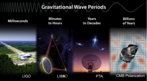
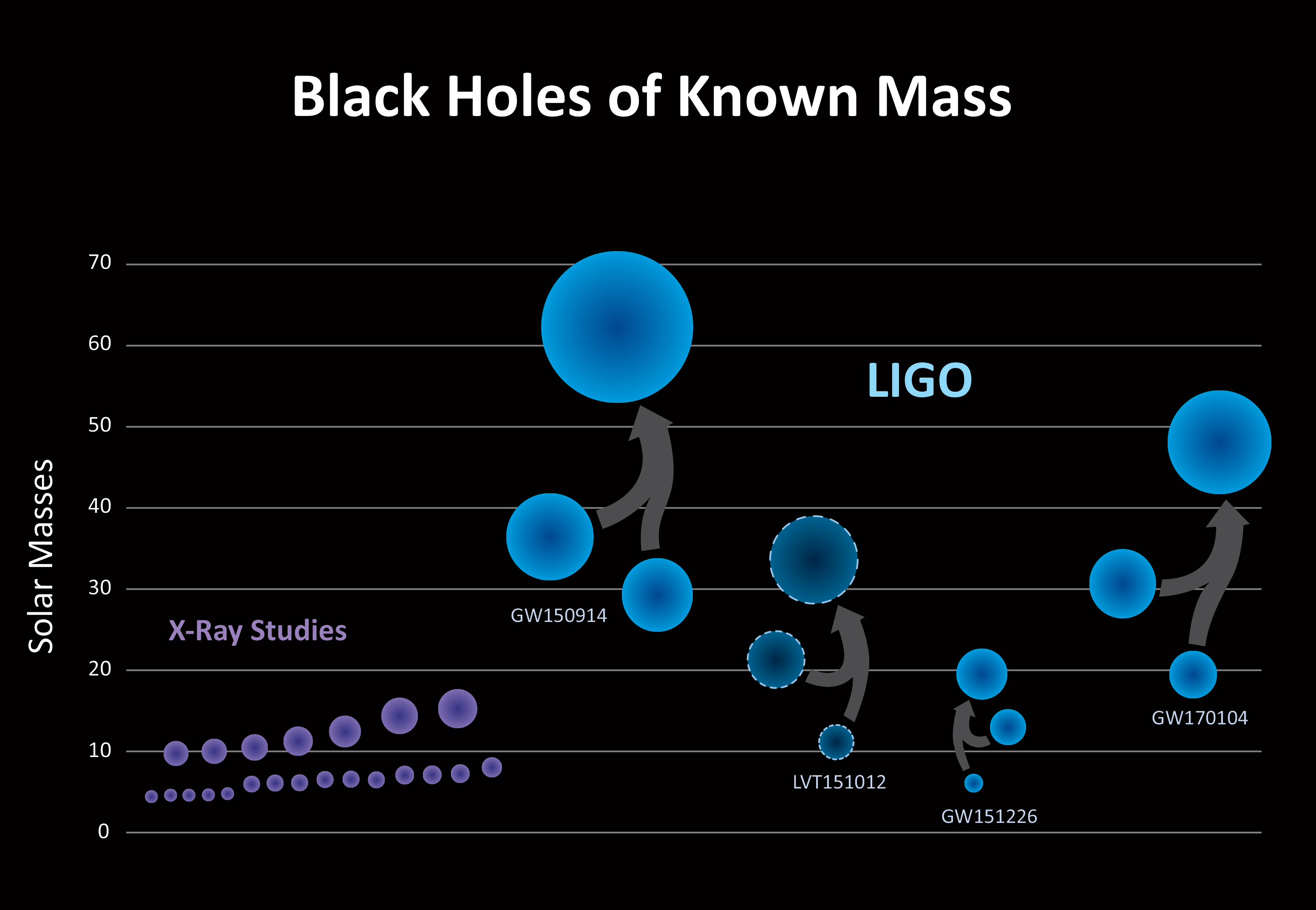
On 14 September 2015, the Laser Interferometer Gravitational-Wave Observatory (LIGO) ushered in a new era in astronomy and astrophysics by opening a part of the gravitational wave spectrum to direct observation. In my 17 February 2017 post,“Perspective on the Detection of Gravitational Waves,” I included the following graphic from an interview of Kip Thorne by Walter Issacson.
 Source: screenshot from Kip Thorne / Walter Issacson interview at: https://www.youtube.com/watch?v=mDFF27Nr-EU
The key point of this graphic is to illustrate how the LIGO detector is able to “see” only a part of the gravitational wave spectrum. The LIGO team reported that the Advanced LIGO detector is optimized for “a range of frequencies from 30 Hz to several kHz, which covers the frequencies of gravitational waves emitted during the late inspiral, merger, and ringdown of stellar-mass binary black holes.” This is the type of event associated with the first several gravitational wave detections. The European Advanced VIRGO detector, which came on line in 2017, operates on the same principle as LIGO, precisely measuring differences in the times-of-flight of laser beams in the two legs of a long baseline interferometer. VIRGO is optimized to view a range of gravitational wave frequencies from about 10 Hz to 10 kHz.
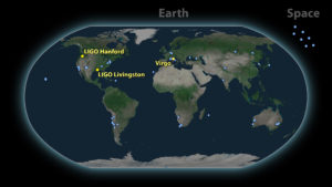
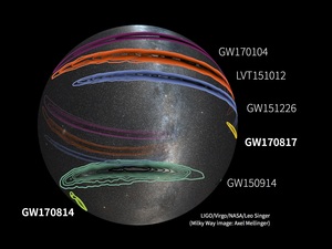
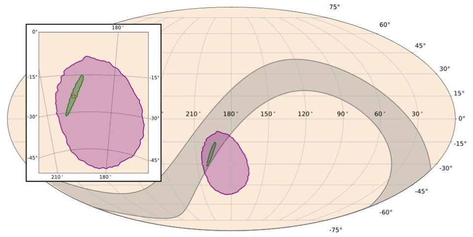
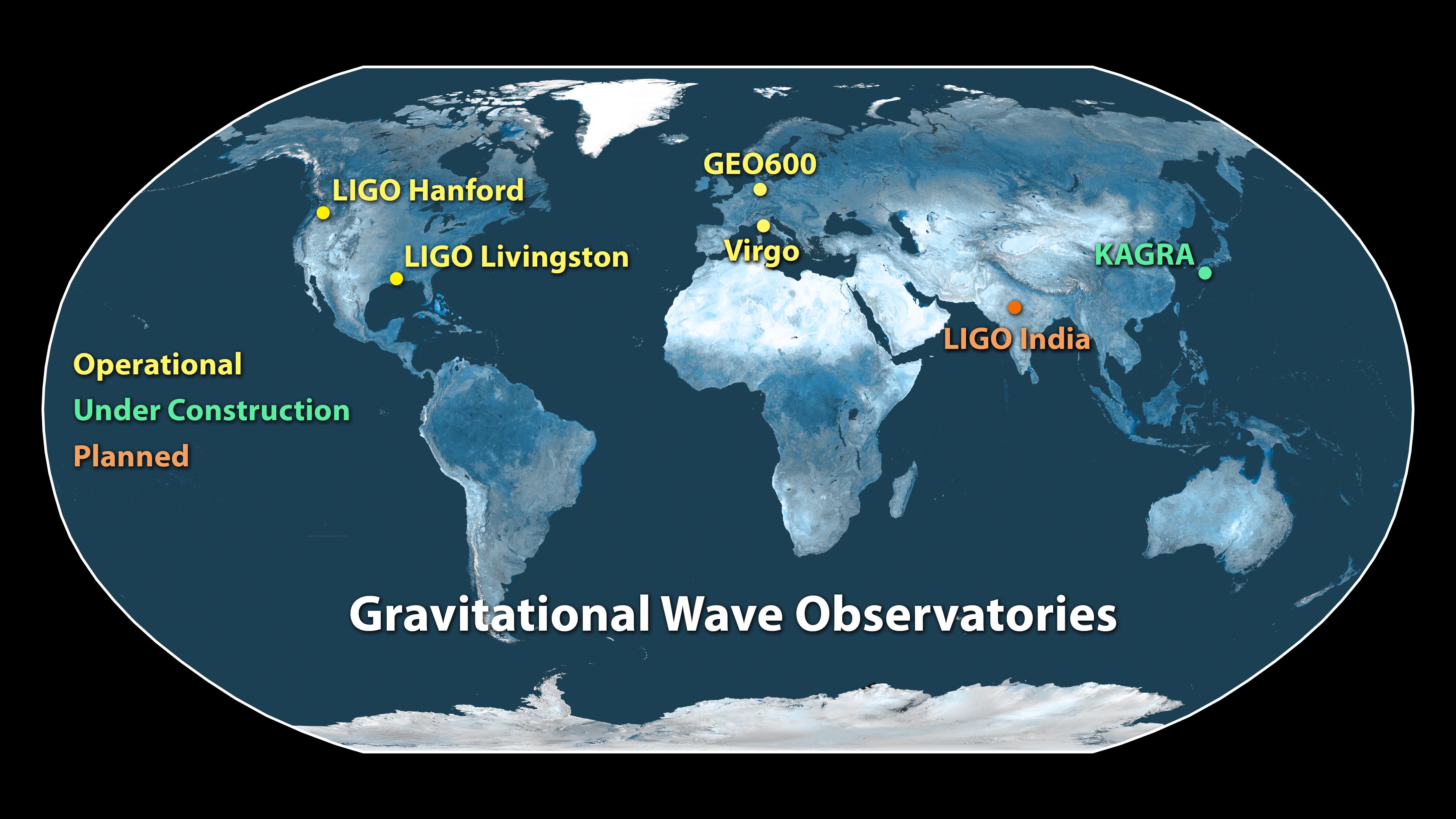
On 17 August 2017, LIGO and VIRGO detected gravitational waves from a different source: the collision of two neutron stars. Unlike the previous gravitational wave detections from black hole coalescence, the neutron star collision that produced GW180817 also produced other observable phenomena in multiple wavelength bands. LIGO and VIRGO triangulated the source of this gravitational wave event, which also was observed by dozens of telescopes on the ground and in space, as shown in the following diagram.
 Source: LIGO – VIRGO, https://www.ligo.org/detections/GW170817/images-GW170817/GW+EM_Observatories.jpg
The ability to cue a worldwide array of multi-spectral observatories on short notice greatly added to the depth of understanding of the GW170817 event. The international collaboration on this event was a great example of the benefits of “multi-messenger” astronomy. For more information, see my 25 October 2017 post, “Linking Gravitational Wave Detection to the Rest of the Observable Spectrum.”
At the 11 April 2018 Lyncean Group meeting, Dr. Rana Adhikari, Professor of Physics, Mathematics and Astronomy at Caltech, provided an update on LIGO in his presentation, “The Dirty Details of Detecting Gravitational Waves from Black Holes.” You can view Dr. Adhikari’s presentation slides at the following link:
https://lynceans.org/talk-119-4-11-18/
As we have seen, the LIGO class of gravitational wave detector is capable of seeing large amplitude, relatively high frequency gravitational waves from very powerful, discrete events: stellar-mass binary black hole coalescence and neutron star collisions.
As shown in the above graphic, viewing lower frequency (longer wavelength) gravitational waves requires different types of detectors, which are discussed below.
LISA – Laser Interferometer Space Antenna
This will be a very long baseline, equilateral triangular laser interferometer in space, established of three spacecraft flying in formation in an Earth-trailing heliocentric orbit. Each leg of the space interferometer will measure 2.5 million kilometers (1.55 million miles), about 625,000 times the length of the LIGO baseline (4 km, 2.49 miles). Each spacecraft will contain a gravitational wave detector sensitive at frequencies from about 10-4 Hz to 10-1 Hz, well below the frequency range of LIGO and VIRGO.
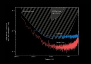
The European Space Agency’s (ESA) LISA Pathfinder spacecraft, which was launched in 2015 and ended its mission in July 2017, validated the technology for the LISA space interferometer.
 Source: ESA, https://www.elisascience.org/
ESA reported:
“Analysis of the LISA Pathfinder mission results towards the end of the mission (red line) compared with the first results published shortly after the spacecraft began science operations (blue line). The initial requirements (top, wedge-shaped area) and that of the future gravitational-wave observatory LISA (middle, striped area) are included for comparison, and show that LISA Pathfinder far exceeded expectations.”
The ESA is planning to launch LISA in the 2029 – 2032 timeframe. See my 27 September 2016 post, “Space-based Gravity Wave Detection System to be Deployed by ESA,” for additional information on LISA. The LISA mission website is at the following link:
PTA – Pulsar Timing Array
A pulsar is a highly magnetized rotating neutron star or white dwarf that emits a beam of electromagnetic radiation. This radiation can be observed only when the beam is pointing toward Earth.
PTA gravitational wave detection is based on correlated radio-telescope observations of an array of many pulsars known as “millisecond pulsars” (MSPs). The signal from an MSP has a very predictable time-of-arrival (TOA), thereby allowing each MSP to function as a galactic “clock.” Small disturbances in each “clock” are measurable with high precision on Earth. In essence, the distance between an MSP and the observing radio-telescope forms one leg of a gravitational wave detector, with the leg length being measured in light-years. A disturbance from a passing gravitational wave would to have a measurable signature across the many MSPs in the pulsar timing array.
A PTA is intended to observe in a different range in gravitational wave frequencies than LIGO and VIRGO, and is expected to see a different category of gravitational wave sources. Whereas LIGO and VIRGO can detect gravitational waves in the tens to thousands of Hz (audio) range, radio-telescope observatories currently are using PTAs to search for gravitational waves in the tens to hundreds of microHertz (10-6Hz) range with prospects of getting down to the 10-8Hz range. The primary source of gravitational waves in this frequency range is expected to be super-massive black hole binaries (billions of solar masses), which are believed to exist throughout the universe at the center of galaxies.
The International Pulsar Timing Array (IPTA) is an international collaboration among the following radio-telescope consortia: European Pulsar Timing Array (EPTA), the North American Nanohertz Observatory for Gravitational Waves (NANOGrav), and the Parkes Pulsar Timing Array (PPTA). The goal of the IPTA is to detect gravitational waves using an array of about 30 MSPs. IPTA reports:
“Using telescopes located around the world is important, because any single telescope can see (a particular) pulsar … for much less than twelve hours, depending on the observing site’s latitude. Thus, the telescopes “trade off” between one another – as the pulsar sets from the perspective of, say, the Parkes telescope in Australia, it rises from the perspective of the Lovell telescope in the UK.”
You’ll find more information on IPTA on their website at the following link:
You can visit the NANOGrav website here:
Continuous gravitational waves
On 10 April 2018, the Max Planck Institute for Gravitational Physics announced the formation of a permanent Max Planck Independent Research Group under the leadership of Dr. M. Alessandra Papa to search for continuous gravitational waves. The primary goal of this research group is to make the first direct detection of gravitational waves from rapidly rotating neutron stars. You can read this announcement here:
http://www.aei.mpg.de/2236875/searchingcontinuouswaves
Generation of the weak, continuous gravitational waves depends on the neutron star having an asymmetry that would perturb the stars gravitational field as it rapidly rotates. The method for detecting these weak, continuous gravitational waves was not described in the Planck Institute announcement.
CMB – Cosmic microwave background
The CBM is believed to be an artifact of the Big Bang and could carry evidence of the primordial gravitational waves from that era. Such evidence would be expected to stretch across broad areas of the observable universe.
The European Space Agency (ESA) developed the Planck space observatory to map the CMB in microwave and infrared frequencies at unprecedented levels of detail. The Planck spacecraft was launched on 14 May 2009 and operated until 23 October 2013. In 2016, the ESA released the results of the Planck all-sky survey of the CBM, which revealed that the universe appears to be isotropic, at least at the resolution of the Planck space observatory. Researchers found that the actual CMB shows only random noise and no signs of patterns.
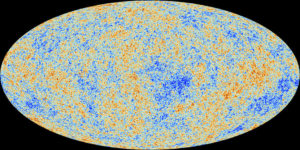 Planck all-sky survey. Source; ESA / Planck Collaboration
You’ll find more information on the Planck mission in my 28 September 2016 post, “The Universe is Isotropic.”
You can access ESA’s Planck science team home page here:
https://www.cosmos.esa.int/web/planck/home
In summary
The North American Nanohertz Observatory for Gravitational Waves (NANOGrav) website contains the following summary chart, which is an alternate view of the chart at the start of this article (from the Kip Thorne / Walter Issacson interview). The NANOGrav chart provides a good perspective on the observational technologies that are opening windows into the broad spectrum of gravitational waves and their varied sources.
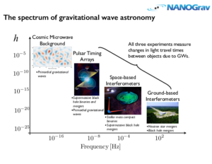
So, in an analogy to the optical spectrum and the range of colors we see every day, the primordial gravitational waves in the CBM would be at the “red” end of the gravitational wave spectrum. The much higher frequency gravitational waves seen by LIGO and VIRGO, from stellar-mass binary black hole coalescence and neutron star collisions, would be at the “violet” end of the gravitational wave spectrum. The LISA space-based interferometer will be looking in the “blue-green” range, while PTA observatories are looking in the “yellow-orange” range.
For more information on the current state of gravitational wave technology, you’ll find a good survey article by Davide Castelvecchia, entitled “Here Come the Waves,” in the 12 April 2018 issue of Nature, which you can read here:
https://www.nature.com/magazine-assets/d41586-018-04157-6/d41586-018-04157-6.pdf


 Source: RAND Corporation, 2019


