Peter Lobner
In my 31 December 2015 post, “Legal Basis Established for U.S. Commercial Space Launch Industry Self-regulation and Commercial Asteroid Mining,” I commented on the likely impact of the “U.S. Commercial Space Launch Competitiveness Act,” (2015 Space Act) which was signed into law on 25 November 2016. A lot has happened since then.
Planetary Resources building technology base for commercial asteroid prospecting
The firm Planetary Resources (Redmond, Washington) has a roadmap for developing a working space-based prospecting system built on the following technologies:
- Space-based observation systems: miniaturization of hyperspectral sensors and mid-wavelength infrared sensors.
- Low-cost avionics software: tiered and modular spacecraft avionics with a distributed set of commercially-available, low-level hardened elements each handling local control of a specific spacecraft function.
- Attitude determination and control systems: distributed system, as above
- Space communications: laser communications
- High delta V small satellite propulsion systems: “Oberth maneuver” (powered flyby) provides most efficient use of fuel to escape Earth’s gravity well
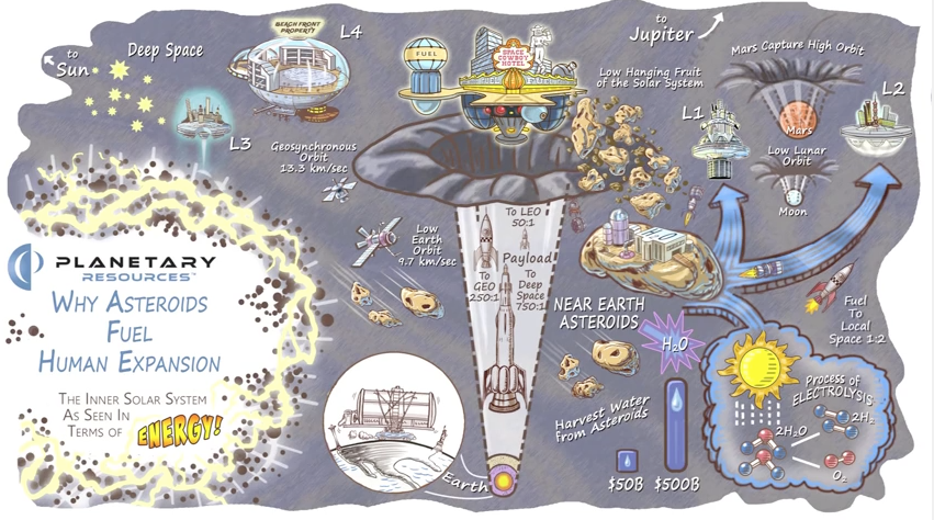
Check out their short video, “Why Asteroids Fuel Human Expansion,” at the following link:
http://www.planetaryresources.com/asteroids/#asteroids-intro
 Source: Planetary Resources
For more information, visit the Planetary Resources home page at the following link:
http://www.planetaryresources.com/#home-intro
Luxembourg SpaceResources.lu Initiative and collaboration with Planetary Resources
On 3 November 2016, Planetary Resources announced funding and a target date for their first asteroid mining mission:
“Planetary Resources, Inc. …. announced today that it has finalized a 25 million euro agreement that includes direct capital investment of 12 million euros and grants of 13 million euros from the Government of the Grand Duchy of Luxembourg and the banking institution Société Nationale de Crédit et d’Investissement (SNCI). The funding will accelerate the company’s technical advancements with the aim of launching the first commercial asteroid prospecting mission by 2020. This milestone fulfilled the intent of the Memorandum of Understanding with the Grand Duchy and its SpaceResources.lu initiative that was agreed upon this past June.”
The homepage for Luxembourg’s SpaceResources.lu Initiative is at the following link:
http://www.spaceresources.public.lu/en/index.html
Here the Grand-Duchy announced its intent to position Luxembourg as a European hub in the exploration and use of space resources.
“Luxembourg is the first European country to set out a formal legal framework which ensures that private operators working in space can be confident about their rights to the resources they extract, i.e. valuable resources from asteroids. Such a legal framework will be worked out in full consideration of international law. The Grand-Duchy aims to participate with other nations in all relevant fora in order to agree on a mutually beneficial international framework.”
Remember the book, “The Mouse that Roared?” Well, here’s Luxembourg leading the European Union (EU) into the business of asteroid mining.
European Space Agency (ESA) cancels Asteroid Impact Mission (AIM)
ESA’s Asteroid Impact Mission (AIM) was planning to send a small spacecraft to a pair of co-orbital asteroids, Didymoon and Didymos, in 2022. Among other goals, this ESA mission was intended to observe the NASA’s Double Asteroid Redirection Test when it impacts Didymoon at high speed. ESA mission profile for AIM is described at the following link:
On 2 Dec 2016, ESA announced that AIM did not win enough support from member governments and will be cancelled. Perhaps the plans for an earlier commercial asteroid mission marginalized the value of the ESA investment in AIM.
Japanese Aerospace Exploration Agency (JAXA) announces collaboration for lunar resource prospecting, production and delivery
On 16 December 2016, JAXA announced that it will collaborate with the private lunar exploration firm, ispace, Inc. to prospect for lunar resources and then eventually build production and resource delivery facilities on the Moon.
ispace is a member of Japan’s Team Hakuto, which is competing for the Google Lunar XPrize. Team Hakuto describes their mission as follows:
“In addition to the Grand Prize, Hakuto will be attempting to win the Range Bonus. Furthermore, Hakuto’s ultimate target is to explore holes that are thought to be caves or “skylights” into underlying lava tubes, for the first time in human history. These lava tubes could prove to be very important scientifically, as they could help explain the moon’s volcanic past. They could also become candidate sites for long-term habitats, able to shield humans from the moon’s hostile environment.”
Hakuto is facing the challenges of the Google Lunar XPRIZE and skylight exploration with its unique ‘Dual Rover’ system, consisting of two-wheeled ‘Tetris’ and four-wheeled ‘Moonraker.’ The two rovers are linked by a tether, so that Tetris can be lowered into a suspected skylight.”

Team Hakuto dual rover. Source: ispace, Inc.
So far, the team has won one Milestone Prize worth $500,000 and must complete its lunar mission by the end of 2017 in order to be eligible for the final prizes. You can read more about Team Hakuto and their rover on the Google Lunar XPrize website at the following link:
http://lunar.xprize.org/teams/hakuto
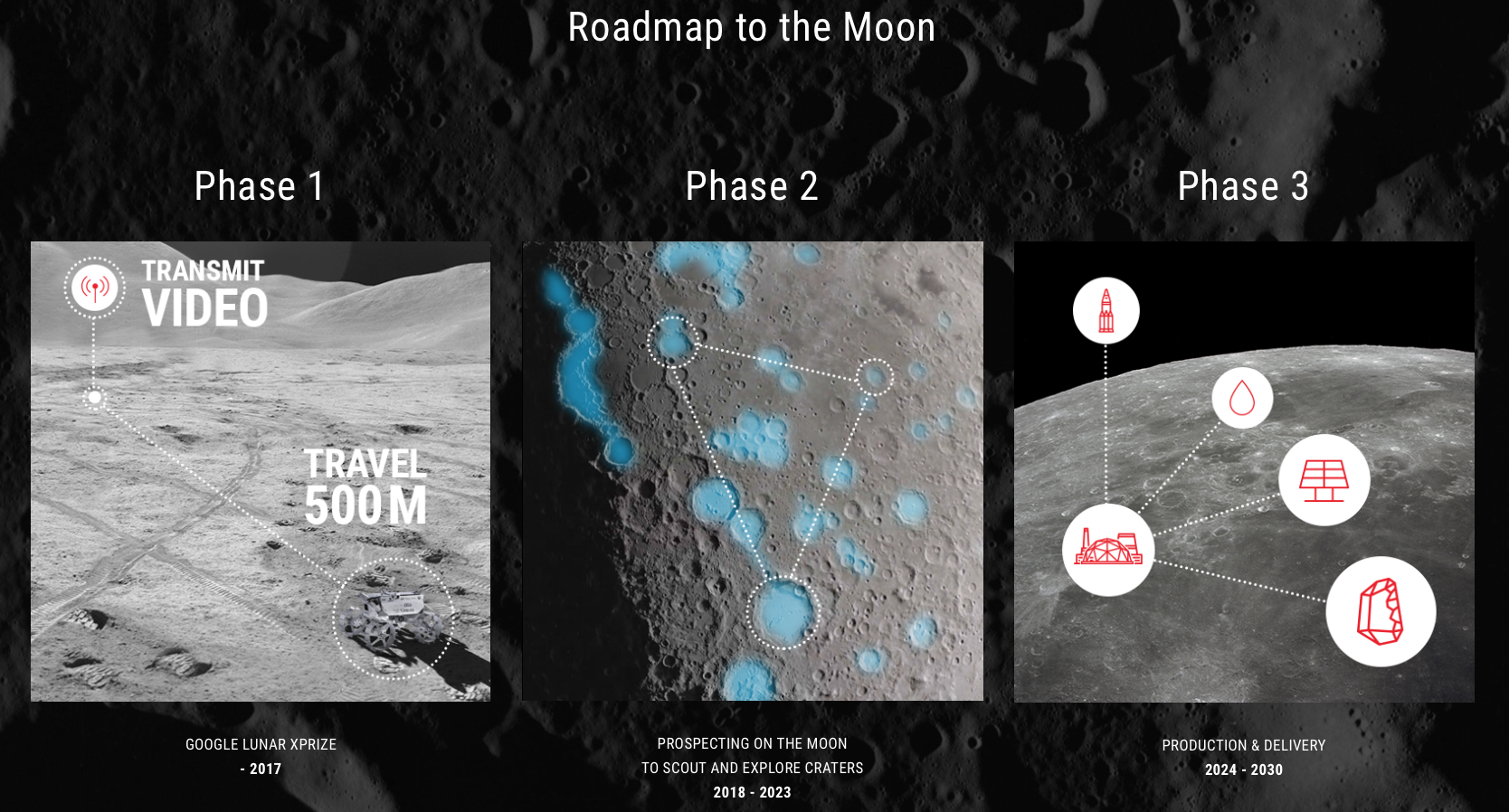
Building on this experience, and apparently using the XPrize rover, ispace has proposed the following roadmap to the moon (click on the graphic to enlarge).
 Source: ispace, Inc.
This ambitious roadmap offers an initial lunar resource utilization capability by 2030. Ice will be the primary resource sought on the Moon. Ispace reports:
“According to recent studies, the Moon houses an abundance of precious minerals on its surface, and an estimated 6 billion tons of water ice at its poles. In particular, water can be broken down into oxygen and hydrogen to produce efficient rocket fuel. With a fuel station established in space, the world will witness a revolution in the space transportation system.”
The ispace website is at the following link:


