The World Air League is the organizer for a monumental airship race around the globe that will be held between September 2023 and May 2024. The World Air League describes their mission as follows:
“The mission and vision of the World Air League are to promote the advancement of lighter-than-air aviation for a sustainable future. The World Air League is creating the World Sky Race as an epic challenge to inspire inventors to invent and adventurers to compete. For strategic impact and purpose, the World Air League in embedding the World Sky Race® to be included in the global educational system to provide the world’s next-generation with a path to explore with their destination an alternate greener, cleaner future.”
The upcoming World Sky Race® will launch in September 2023 when the competing airships cross the Prime Meridian heading east over Greenwich, London, and will end eight months later in Paris in May 2024, after the competitors have circumnavigated the globe. During the eight-month race, the airships will be flying over 130+ UNESCO World Heritage Sites and cities. Hopefully this flying caravan will inspire people worldwide to the green transportation opportunities represented by modern airships. The following map shows the proposed route.
Source: World Air League
The following travel poster images provide inspiring views of some of the destinations that will be visited during the upcoming World Sky Race®.
Source: World Air League
The World Air League previously attempted to organize the inaugural World Sky Race® in 2010. That race didn’t occur. Hopefully the planned 2023 – 2024 race will become a reality and will be a rousing success.
Update, 26 October 2024:
The World Sky Race didn’t occur as scheduled and new dates for the event haven’t been announced. However, viable airship candidates for around-the-world flight are being developed and, in 2024, two airship manufacturers announced their plans for around-the-world flights later in this decade. Maybe there will be a World Sky Race in the future.
This article provides a brief overview of the “mainstream” international plans to deliver the first large tokamak commercial fusion power plant prototype in the 2060 to 2070 timeframe. Then we’ll take a look at alternate plans that could lead to smaller and less expensive commercial fusion power plants being deployed much sooner, perhaps in the 2030s. These alternate plans are enabled by recent technical advances and a combination of public and private funding for many creative teams that are developing and testing a diverse range of fusion machines that may be developed in the near-term into compact, relatively low-cost fusion power plants.
1. Plodding down the long road to controlled nuclear fusion with ITER
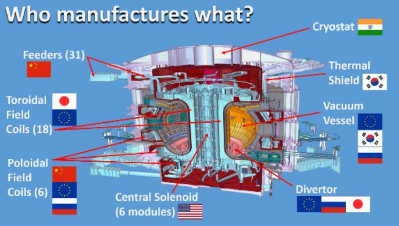
Mainstream fusion development is focused on the construction of the International Thermonuclear Experimental Reactor (ITER), which is a very large magnetic confinement fusion machine. The 35-nation ITER program describes their reactor as follows: “Conceived as the last experimental step to prove the feasibility of fusion as a large-scale and carbon-free source of energy, ITER will be the world’s largest tokamak, with ten times the plasma volume of the largest tokamak operating today.” ITER is intended “to advance fusion science and technology to the point where demonstration fusion power plants can be designed.”
ITER is intended to be the first fusion experiment to produce a net energy gain (“Q”) from fusion. Energy gain is the ratio of the amount of fusion energy produced (Pfusion) to the amount of input energy needed to create the fusion reaction (Pinput). In its simplest form, “breakeven” occurs when Pfusion = Pinput and Q = 1.0. The highest value of Q achieved to date is 0.67, by the Joint European Torus (JET) tokamak in 1997.The ITER program was formally started with the ITER Agreement, which was signed on 21 November 2006.
Nations contributing to the manufacture of major ITER components. Source: SciTechDaily (28 Jul 2020)
The official start of the “assembly phase” of the ITER reactor began on 28 July 2020. The target date of “first plasma” currently is in Q4, 2025. At that time, the reactor will be only partially complete. During the following ten years, construction of the reactor internals and other systems will be completed along with a comprehensive testing and commissioning program. The current goal is to start experiments with deuterium / deuterium-tritium (D/D-T) plasmas in December 2035.
After initial experiments in early 2036, there will be a gradual transition to fusion power production over the next 12 – 15 months. By mid-2037, ITER may be ready to conduct initial high-power demonstrations, operating at several hundred megawatts of D-T fusion power for several tens of seconds. This milestone will be reached more than 30 years after the ITER Agreement was signed.
Subsequent experimental campaigns will be planned on a two-yearly cycle. The principal scientific mission goals of the ITER project are:
Produce 500 MW of energy from fusion while using only 50 MW of energy for input heating, yielding Q ≥ 10
Demonstrate Q ≥ 10 for burn durations of 300 – 500 seconds (5.0 – 8.3 minutes)
Demonstrate long-pulse, non-inductive operation with Q ~ 5 for periods of up to 3,000 seconds (50 minutes).
All that energy will get absorbed in reactor structures, with some of it being carried off in cooling systems. However, ITER will not generate any electric power from fusion.
The total cost of the ITER program currently is estimated to be about $22.5 billion. In 2018, Reuters reported that the US had given about $1 billion to ITER so far, and was planning to contribute an additional $500 million through 2025. In Fiscal Year 2018 alone, the US contributed $122 million to the ITER project.
You’ll find more information on the ITER website, including a detailed timeline, at the following link: https://www.iter.org
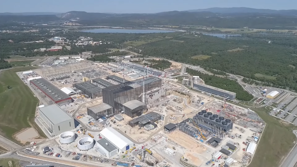
The ITER site in 2020, being built next to the Cadarache facility in Saint-Paul-lès-Durance, in Provence, southern France. Source: Macskelek via Wikipedia
2. Timeline for a commercial fusion power plant based on ITER
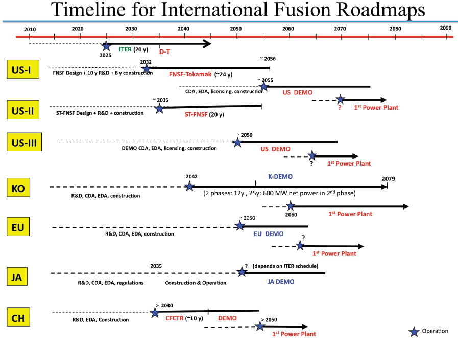
In December 2018, a National Academy of Sciences, Engineering & Medicine (NASEM) committee issued a report that included the following overview of timelines for fusion power deployment based on previously studied pathways for developing fusion power plants derived from ITER. The timelines for the USA, South Korea, Europe, Japan and China are shown below.
Source: “A Strategic Plan for U.S. Burning Plasma Research” (NASEM, 2019)
All of the pathways include plans for a DEMO fusion power plant (i.e., a prototype with a power conversion system) that would start operation between 2050 and 2060. Based on experience with DEMO, the first commercial fusion power plants would be built a decade or more later. You can see that, in most cases, the first commercial fusion power plant is not projected to begin operation until the 2060 to 2070 timeframe.
3. DOE is helping to build a fork in the road
Fortunately, a large magnetic confinement tokamak like ITER is not the only route to commercial fusion power. However, ITER currently is consuming a great deal of available resources while the promise of fusion power from an ITER-derived power plant remains an elusive 30 years or more away, and likely at a cost that will not be commercially viable.
Since the commitment was made in the early 2000s to build ITER, there have been tremendous advances in power electronics and advanced magnet technologies, particularly in a class of high temperature superconducting (HTS) magnets known as rare-earth barium copper oxide (REBCO) magnets that can operate at about 90 °K (-297 °F), which is above the temperature of liquid nitrogen (77 °K; −320 °F). These technical advances contribute to making ITER obsolete as a path to fusion power generation.
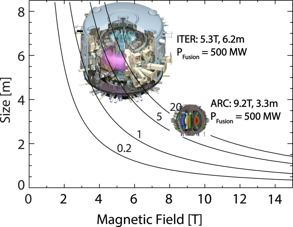
A 2019 paper by Martin Greenwald describes the relationship of constant fusion gain (Q = Pfusion / Pinput) to the magnetic field strength (B) and the plasma radius (R) of a tokamak device. As it turns out, Q is proportional to the product of B and R, so, for a constant gain, there is a tradeoff between the magnetic field strength and the size of the fusion device. This can be seen in the comparison between the relative field strengths and sizes of ITER and ARC (a tokomak being designed now), which are drawn to scale in the following chart.
Contours of constant fusion gain (Q) plotted against magnetic field strength (T, Tesla) and device size (plasma radius in meters): Source: Greenwald (2019)
ITER has lower field strength conventional superconducting magnets and is much larger than ARC, which has much higher field strength HTS magnets that enable its compact design. Greenwald explains, “With conventional superconductors, the region of the figure above 6T was inaccessible; thus, ITER, with its older magnet technology, is as small as it could be.” So, ITER will be a big white elephant, useful for scientific research, but likely much less useful on the path to fusion power generation than anyone expected when they signed the ITER Agreement in 2006.
For the past decade, there has been increasing interest in, and funding for, developing lower cost, compact fusion power plants using any fusion technology that can deliver a useful power generation capability at an commercially viable cost. Department of Energy’s (DOE) Advanced Research Project Agency – Energy (ARPA-E) has recommended the following cost targets for such a commercial fusion power plant:
Overnight capital cost of < US $2 billion and < $5/W
At $5/W, the upper limit would be a 400 MWe fusion power plant.
Since 2014, DOE has created a series of funding programs for fusion R&D projects to support development of a broad range of compact, low-cost fusion power plant design concepts. This was a significant change for the DOE fusion program, which has been contributing to ITER and a whole range of other fusion-related projects, but without a sense of urgency for delivering the technology needed to develop and operate commercial fusion power plants any time soon. Now, a small part of the DOE fusion budget is focused on resolving some of the technical challenges and de-risking the path forward sooner rather than later, and thereby improving the investment climate to the point that investors become willing to contribute to the development of small, low-cost fusion power plants that may be able to produce electrical power within the next decade or two.
These DOE R&D programs are administered ARPA-E and the Office of Science, Fusion Energy Sciences (FES).
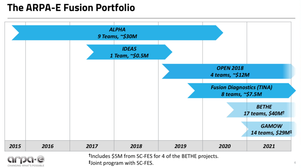
ARPA-E advances high-potential, high-impact energy technologies that are too early for private-sector investment. The ARPA-E fusion R&D programs are named ALPHA, IDEAS, BETHE, TINA and GAMOW. ARPA-E jointly funds the GAMOW fusion R&D program and part of the BETHE program with FES. In addition, the ARPA-E OPEN program makes R&D investments in the entire spectrum of energy technologies, including fusion.
FES is the largest US federal government supporter of research that is addressing the remaining obstacles to commercial fusion power. The FES fusion R&D program is named INFUSE. In addition FES jointly funds GAMOW and part of BETHE with ARPA-E.
Here’s an overview of these DOE programs.
DOE ARPA-E ALPHA program (2015 – 2020)
In 2015, ARPA-E initiated a five-year, $30 million research program into lower-cost approaches to producing electric power from fusion. This was known as the ALPHA program (Accelerating Low-Cost Plasma Heating and Assembly). The goal was to expand the range of potential technical solutions for generating power from fusion, focusing on small, low-cost, pulsed magneto-inertial fusion (MIF) devices.
There were nine program participants in the ALPHA program. Helion Energy ($3.97 million) and MIFTI ($4.60 million) were among the private fusion reactor firms receiving ALPHA awards. Los Alamos National Laboratory (LANL) received $6.63 million to fund the Plasma Liner Experiment (PLX-α) team, which included the private firm HyperV Technologies Corp.
In 2018, ARPA-E asked JASON to assess its accomplishments on the ALPHA program and the potential of further investments in this field. Among their findings, JASON reported that MIF is a physically plausible approach to controlled fusion and, in spite of very modest funding to date, some particular approaches are within a factor of 10 of scientific break-even. JASON also recommended supporting all promising approaches, while giving near-term priority to achieving breakeven (Q ≥ 1) in a system that can be scaled up to be commercial power plant. You can read the November 2018 JASON report here: https://fas.org/irp/agency/dod/jason/fusiondev.pdf
DOE ARPA-E IDEAS program (2017 – 2019)
The ARPA-E IDEAS program (Innovative Development in Energy-Related Applied Science) provides support of early-stage applied research to explore pioneering new concepts with the potential for transformational and disruptive changes in any energy technology. IDEAS awards are restricted to a maximum of $500,000 in funding. There have been 59 IDEAS awards for a broad range of energy-related technologies, largely to national laboratories and universities.
There was one fusion-related IDEAS award to the University of Washington ($482 k).
DOE ARPA-E OPEN program (2018)
In 2018, ARPA-E issued its fourth OPEN funding opportunity designed to catalyze transformational breakthroughs across the entire spectrum of energy technologies, including fusion. OPEN 2018 is a $199 million program funding 77 projects.
Four fusion-related projects were funded for a total of about $12 million. ZAP Energy ($6.77 million), CTFusion ($3.0 million) and Princeton Fusion Systems ($1.1 million) were among the private fusion reactor firms receiving OPEN 2018 awards.
DOE ARPA-E TINA Fusion Diagnostics program (2019 – 2021)
The TINA program established diagnostic “capability teams” to support state-of-the-art diagnostic system construction/deployment and data analysis/interpretation on ARPA-E-supported fusion experiments. This program awarded $7.5 million to eight teams, primarily from national laboratories and universities.
DOE ARPA-E BETHE program (2020 – 2024)
DOE’s ARPA-E also runs the BETHE program (Breakthroughs Enabling THermonuclear-fusion Energy), which is a $40 million program that aims to deliver a large number of lower-cost fusion concepts at higher performance levels. BETHE R&D is focused in the following areas:
Concept development to advance the performance of inherently lower cost but less mature fusion concepts.
Component technology development that could significantly reduce the capital cost of higher cost, more mature fusion concepts.
Capability teams to improve/adapt and apply existing capabilities (e.g., theory/modeling, machine learning, or engineering design/fabrication) to accelerate the development of multiple concepts.
ZAP Energy ($1 million) and Commonwealth Fusion Systems ($2.39 million) were among the private fusion reactor firms directly receiving BETHE awards.
The following awards were made to universities or national laboratories working with teams that include a significant role for a private fusion reactor firm:
University of Washington received $1.5 million for improving IDCD plasma control, which is applicable to their collaborative work with CTFusion on the Dynomak fusion reactor concept.
LANL received $4.62 million to fund the Plasma Liner Experiment (PLX-α) team, which includes HyperJet
DOE ARPA-E / FES GAMOW program (2020 – 2024)
Yet another DOE funding program for fusion research is named GAMOW (Galvanizing Advances in Market-Aligned Fusion for an Overabundance of Watts), which is a $29 million program announced in February 2020. GAMOW is jointly funded and overseen by ARPA-E and FES. GAMOW program focuses on the following three areas:
Technologies and subsystems between the fusion plasma and balance of plant.
Princeton Fusion Systems ($1.1 million) was among the private fusion reactor firms receiving GAMOW awards.
DOE FES INFUSE program (2020 – present)
The DOE FES INFUSE program (Innovation Network for Fusion Energy) was created to “accelerate fusion energy development in the private sector by reducing impediments to collaboration involving the expertise and unique resources available at DOE laboratories.” ….”DOE-FES will accept basic research applications focused on innovation that support production and utilization of fusion energy (e.g., for generation of electricity, supply of process heat, etc.)….”
In Fiscal Years 2020 and 2021, the INFUSE program annual budget was $4 million. INFUSE is a cost sharing program with DOE-FES funding 80% of a project’s cost and the award recipient funding the remaining 20%. The DOE-FES INFUSE program home page is here: https://infuse.ornl.gov
So far, there have been three rounds of INFUSE awards. I think you will find that it is much more difficult to find detailed information on the DOE FES INFUSE awards, which are administered by Oak Ridge National Laboratory (ORNL), than it is to find information on any of the DOE ARPA-E program. Here’s a brief INFUSE summary.
1st round FY 2020: On 15 October 2019, DOE announced the first INFUSE awards, which provided funding for 12 projects with representation from six private companies partnering with six national laboratories. The six private firms included: Commonwealth Fusion Systems (4 awards) and TAE Technologies, Inc. (3 awards)
2nd round FY 2020: On 3 September 2020, DOE announced funding for 10 projects. The private firms included: Commonwealth Fusion Systems (3 awards), TAE Technologies, Inc. (1 award), Tokamak Energy, Inc. (UK, 3 awards), and General Fusion Corp. (Canada, 1 award).
1st round FY 2021: On 3 December 2020, DOE announced funding 10 projects in a second round of FY 2021 INFUSE awards. The private firms receiving awards included: Commonwealth Fusion Systems (1 award), General Fusion Corp. (Canada, 1 award), MIFTI (1 award), Princeton Fusion Systems (1 award), TAE Technologies, Inc. (2 awards), Tokamak Energy, Inc. (UK, 2 awards).
DOE-FES has issued a call for new proposals for FY 2021 INFUSE awards. The closing date for submissions is 26 February 2021.
So far, these ARPA-E and FES programs have committed about $127 million in public funds to 77 different projects between 2014 and 2021. While some of the awards are sizeable ($5 – 6 million), many are very modest awards. The DOE total for all small (non-mainstream) fusion projects over a seven year period is about the same amount as the annual US contribution to the ITER program, which isn’t going lead to a fusion power plant in my lifetime, if ever.
While DOE has been kind enough to create the fork in the road, they do not have the deployable financial resources to push on to the next step of actually building prototypes of commercial fusion power plants in the near term.
4. A roadmap for achieving commercial fusion sooner
In 2019 and 2021, the National Academies and DOE-FES, respectively, published the recommendations of committees that were charged with defining the path(s) forward for the US to achieve commercial fusion power. In both cases, the committee recommended continued support for ITER while urging the US to proceed with a separate national program that encourages and supports public-private partnerships to build compact power plants that produce electricity from fusion at the lowest possible capital cost. These committee reports are briefly summarized below.
National Academies: “Final Report of the Committee on a Strategic Plan for U.S. Burning Plasma Research” (2019)
In December 2018, a National Academy of Sciences, Engineering & Medicine (NASEM) committee issued a report entitled, “A Strategic Plan for U.S. Burning Plasma Research.”
As noted previously, the NASEM report described the current path forward based on power plants derived largely from ITER technology. On this path, the first commercial fusion power plant is not projected to begin operation until the 2060 to 2070 timeframe.
The NASEM committee report is very important because it defines an alternate pathway (i.e., the fork in the road) that could deliver fusion power considerably sooner and at much lower capital cost.
The committee offered the following recommendations:
The US should remain an ITER partner. This is the most cost-effective way to gain experience with burning plasma at the scale of a power plant. However:
Significant R&D is required in addition to ITER to produce electricity from this type of fusion reactor.
ITER is too large and expensive to be economically competitive in the US market when compared to other carbon-neutral energy technologies.
The US should start a national program of accompanying research and technology leading to the construction of a compact pilot power plant that produces electricity from fusion at the lowest possible capital cost.
Effective application of US near-term R&D investments is critical, as other nations continue to invest in new fusion facilities that advance their own approaches.
DOE FES: “Powering the Future – Fusion & Plasmas” (2021)
In January 2021, DOE FES published a draft report from their Fusion Energy Sciences Advisory Committee (FESAC) entitled “Powering the Future – Fusion & Plasmas.” This draft report supports the NASEM committee recommendations and concluded that there are two viable paths to commercial fusion power:
Partnership in the ITER fusion project is essential for US fusion energy development, as is supporting the continued growth of the private sector fusion energy industry.
Public-private partnerships have the potential to reduce the time required to achieve commercially viable fusion energy.
The fusion pilot plant goal requires “a pivot toward research and development of fusion materials and other needed technology.” Several new experimental facilities were recommended.
As of late January 2021, the FESAC final report was in preparation. When available, it will be posted here: http://usfusionandplasmas.org
Funding at the fork in the road
At the fork in the road, the US will be hedging its bets and taking both paths, continuing to support ITER at the current level (about $125 million/year) while building new fusion experimental facilities and trying to place a stronger emphasis on timely development of compact fusion power plants through public-private partnerships as well as infusions of private capital.
In the years ahead, the DOE FES fusion budget is expected to be essentially flat, with growth at just a modest rate of 2%/year being among the likely range of budget scenarios. At the same time, FES will attempt to launch several new major fusion R&D facilities and related programs, as recommended by FESAC.
Without a significantly bigger budget authorization from Congress, the FES budget becomes a zero sum game. To create the budget for any of these new R&D facilities and programs, other part of the FES budget have to lose. In this constrained budget environment, I think FES funding for compact fusion power plant development will find stiff competition and will not be on a growth path.
Recall that ARPA-E’s role is to advance high-potential, high-impact energy technologies that are too early for private-sector investment. When major risk issues for a particular fusion reactor concept have been resolved to an appropriate level, funding from ARPA-E may be redirected to other higher risk matters waiting to be addressed.
While the NASEM and FESAC reports support public-private partnerships, the sheer magnitude of the funds required (many billions of dollars) to develop several small prototype fusion power plant designs in parallel exceeds DOE’s ability to fund the deals at the same level as the current 80% (DOE) / 20% (private) partnership deals. The FES annual budget for the past three years has been quite modest: $564 million (FY2019 enacted), $671 million (FY2020 enacted) and $425 million (FY2021 requested).
Making real progress toward deployment of operational fusion power plants will depend on billions of dollars in private / institutional capital being invested in the firms that will design and build the first small commercial fusion power plants.
I think DOE and the commercial fusion power industry are in a similar position to NASA and the commercial spaceflight industry two decades ago when Blue Origin (Jeff Bezos, 2000) and SpaceX (Elon Musk, 2002) were founded. At that time, the traditional route to space was via NASA. Two decades later, it’s clear that many commercial firms and their investors have contributed to building a robust low Earth orbit spaceflight industry that could never have been developed in that short time frame with NASA’s limited budget. In the next two decades, I think the same type of transition needs to occur in the relationship between DOE and the private sector fusion industry if we expect to reap the benefits of clean fusion power soon. It’s time for FES and the commercial fusion industry to confirm that they share a vision and a common aggressive timeline for bringing small commercial fusion power plants to the market. That point doesn’t come across in the FESAC report.
Private and institutional investors already making major investments in the emerging fusion energy market. As you might expect, some fusion firms have been much more successful than others in raising funds. You’ll find a summary of publically available funding information on the Fusion Energy Base website here: https://www.fusionenergybase.com/organization/commonwealth-fusion-systems
5. The US Navy also may be building a fork in the road
The Navy has been quietly developing its own concepts for compact fusion power plants. We’ll take a look at three recent designs. Could the Navy wind up being an important contributor to the development and deployment of commercial fusion power plants?
6. The race is on to beat ITER with smaller, lower-cost fusion
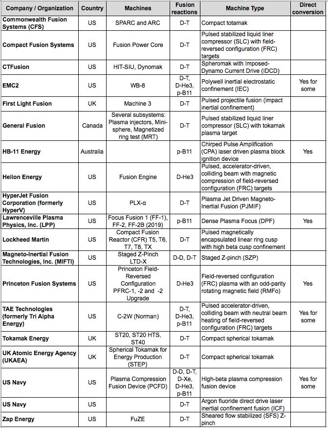
In this section, we’ll take a look at the status of the following small fusion power plant development efforts, mostly by private companies.
Collectively, they are applying a diverse range of technologies to the challenge of generating useful electric power from fusion at a fraction of the cost of ITER. Based on claims from the development teams, it appears that some of the compact fusion reactor designs are quite advanced and probably will be able to demonstrate a net energy gain (Q > 1.0) in the 2020s, well before ITER.
You’ll find details on these 18 organizations and their fusion reactor concepts in my separate articles at the following links:
There certainly are many different technical approaches being developed for small, lower-cost fusion power plants. Several teams are reporting encouraging performance gains that suggest that their particular solutions are on credible paths toward a fusion power plant. However, as of January 2021, none of the operating fusion machines have achieved breakeven, with Q = 1.0, or better. It appears that goal remains at least a few years in the future, even for the most advanced contenders.
The rise of private funding and public-private partnerships is rapidly improving the resources available to many of the contenders. Good funding should spur progress for many of the teams. However, don’t be surprised if one or more teams wind up at a technical or economic dead end that would not lead to a commercially viable fusion power plant. Yes, I think ITER is heading down one of those dead ends right now.
So, where does that leave us? The promise for success with a small, lower-cost fusion power plant is out there, and such power plants should win the race by a decade or more over an ITER-derived fusion power plant. While there are many contenders, which ones are the leading contenders for deploying a commercially viable fusion power plant?
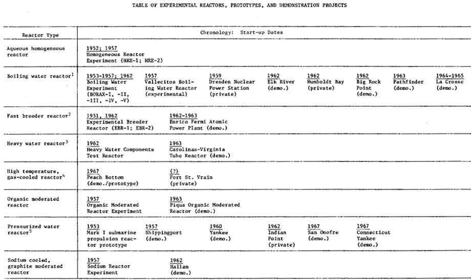
To give some perspective, it’s worth taking a moment to recall the earliest history of the US commercial nuclear power industry, which is recounted in detail for the period from 1946 – 1963 by Wendy Allen in a 1977 RAND report and summarized in the following table.
US fission demonstration power plants. Source: RAND R-2116-NSF
The main points to recognize from the RAND report are:
Eight different types of fission reactors were built as demonstration plants and tested. All of the early reactors were quite small in comparison to later nuclear power plants.
Some were built on Atomic Energy Commission (AEC, now DOE) national laboratory sites and operated as government-owned proof-of-principle reactors. The others were licensed by the AEC (now the Nuclear Regulatory Commission, NRC) and operated by commercial electric power utility companies. These reactors were important for building the national nuclear regulatory framework and the technical competencies in the commercial nuclear power and electric utility industries.
In the long run, only two reactor designs survived the commercial test of time and proved their long-term financial viability: the pressurized water reactor (PWR) and the boiling water reactor (BWR), which are the most common types of fission power reactors operating in the world today.
With the great variety of candidate fusion power plant concepts being developed today, we simply don’t know which ones will be the winners in a long-term competition, except to say that an ITER-derived power plant will not be among the winners. What we need is a national demonstration plant program for small fusion reactors. This means we need the resources to build and operate several different fusion power reactor designs soon and expect that the early operating experience will quickly drive the evolution of the leading contenders toward mature designs that may be successful in the emerging worldwide market for fusion power. The early fission reactor history shows that we should expect that some of the early fusion power plant designs won’t survive in the long-term fusion power market, for a variety of reasons.
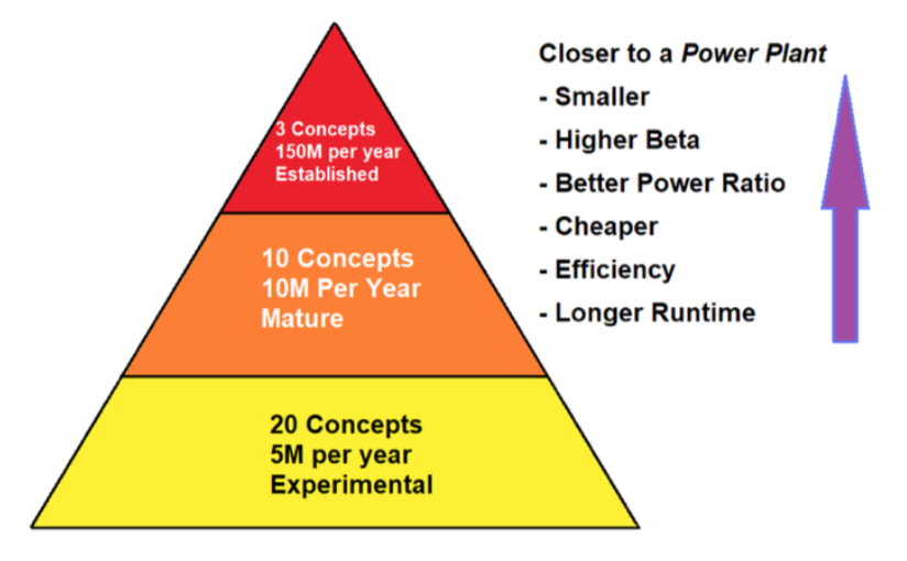
Matthew Moynihan, in his 2019 article, “Selling Fusion in Washington DC,” on The Fusion Podcast website, offered the following approach, borrowed from the biotech industry, to build a pipeline of credible projects while driving bigger investments into the more mature and more promising programs. Applying this approach to the current hodgepodge of DOE fusion spending would yield more focused spending of public money toward the goal of delivering small fusion power plants as soon as practical. The actual dollar amounts in the following chart can be worked out, but I think the basic principle is solid.
Source: The Fusion Podcast, 12 January 2019
With this kind of focus from DOE, the many contenders in the race to build a small fusion power plant could be systematically ranked on several parameters that would make their respective technical and financial risks more understandable to everyone, especially potential investors. With an unbiased validation of relative risks from DOE, the leading candidates in the US fusion power industry should be able to raise the billions of dollars that will be needed to develop their designs into the first wave of demonstration fusion power plants, like the US fission power industry did 60 to 70 years ago.
Perhaps Carly Anderson had the right idea when she suggested Fantasy Fusion as a way to introduce some fun into the uncertain world of commercial fusion power development and investment. You can read her September 2020 article here: https://medium.com/prime-movers-lab/fantasy-fusion-77621cc901e2
If you believe we’re coming into the home stretch, it’s not too late to place a real bet by actually investing in your favorite fusion team(s). It is risky, but the commercial fusion power trophy will be quite a prize! I’m sure it will come with some pretty big bragging rights.
C. L. Nehi, et al., “Retrospective of the ARPA-E ALPHA Fusion Program,” Journal of Fusion Energy, 38_506 – 521, 2019: https://www.osti.gov/biblio/1572943
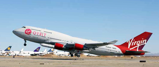
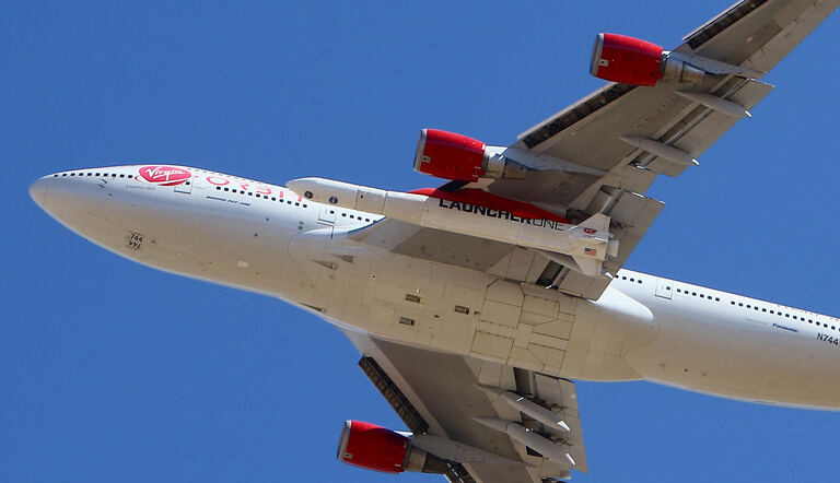
On 17 January 2021, Virgin Orbit conducted an airborne launch from their modified Boeing 747-400 “mothership,” Cosmic Girl, and their LauncherOne rocket boosted a payload of 10 small CubeSats into low Earth orbit. This marks the first commercial orbital mission for Virgin Orbit.
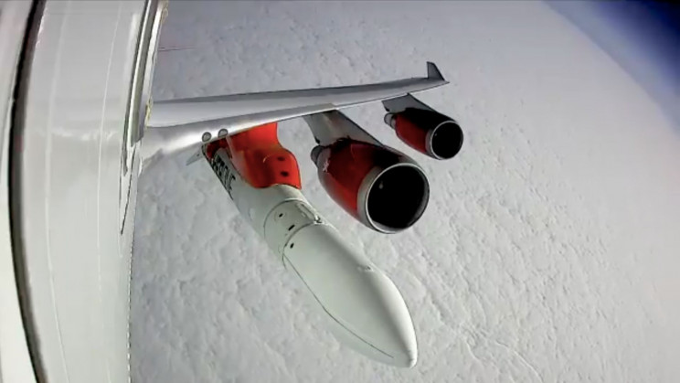
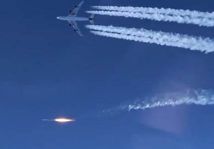
Cosmic Girl carrying a LauncherOne rocket takes off from Mojave Air and Space Port.Source: Virgin Orbit (above), AP Photo/Matt Hartman (below)Cosmic Girl performs the pre-launch pitch-up maneuver at an altitude of about 35,000 ft (10,688 m) during a test flight test on 12 April 2020. Source, three photos above: Virgin OrbitLaunch 17 January 2021. Source: Virgin Orbit
LauncherOne is a 70 foot long (21.34 meter), liquid fueled, two stage booster rocket that can deliver a 300 to 500 kg (661 to 1,102 lb) satellite payload to orbit. Due to the flexibility of using an airborne launch platform, the satellite can be placed into an orbit at any inclination between 0° (equatorial) to 120° (30° retrograde).
NASA sponsored the 10 CubeSats launched on 17 January under their Educational Launch of Nanosatellites (ELaNa) program. NASA also funded the launch under its Venture Class Launch Services (VCLS) program.
This was Virgin Orbit’s second attempt to launch satellites into orbit with LauncherOne. The first flight on 25 May 2020 failed due to a break in a propellant line for the first stage engine.
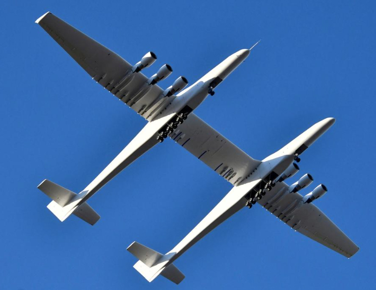
After Paul Allen’s death on 15 October 2018, the focus of Stratolaunch changed dramatically and Roc has remained grounded at the Mojave Air and Space Port since its first flight.
Roc on its first flight. Source: REUTERS/Gene Blevins/File Photo
It appears that, on 11 October 2019, Stratolaunch Systems was sold by its original holding company, Vulcan Inc., to an undisclosed new owner. Since then, Stratolaunch has put increased emphasis on using the Roc as an airborne launch platform for testing hypersonic vehicles. On 10 November 2020, Alan Boyle, writing for GeekWire , reported, “Today, Stratolaunch announced that it’s partnering with an aerospace research and development company called Calspan to build and test models of its Talon-A hypersonic vehicle, a reusable prototype rocket plane.”
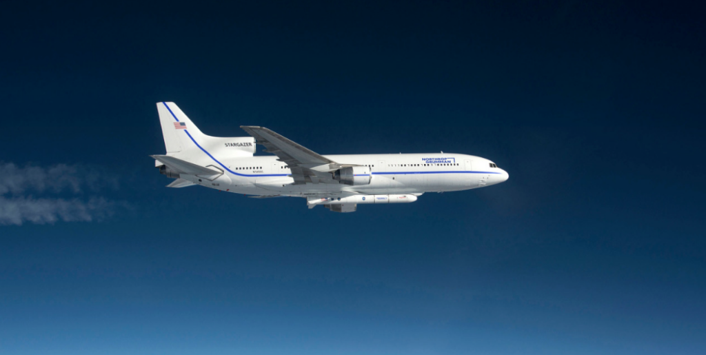
Since 1990, Northrop Grumman Innovation Systems (formerly Orbital ATK and before that Orbital Sciences Corporation) has offered airborne launch services with their converted Stargazer L-1011 mothership and Pegasus booster rocket. From a launch altitude of about 40,000 ft (12,192 m), a three-stage Pegasus XL can carry satellites weighing up to 1,000 pounds (453.59 kg) into low-Earth orbit.
The L-1011 Stargazer carrying a Pegasus XL rocket. Source: Northrop Grumman
A year ago, this might have seemed like a foolish question. An autonomous car racing in the Indianapolis 500 Mile Race? Ha! When pigs fly!
The Indy 500 Borg Warner Trophy. Source: The359 – Flickr via Wikipedia
One of the first things you may notice about the Borg Warner Trophy is that the winning driver of each Indy 500 Race is commemorated with a small portrait/sculpture of their face in bas-relief along with a small plaque with their name, winning year and winning average speed. Today, 105 faces grace the trophy.
Borg Warner Trophy close-up. Source: WISH-TV, Indianapolis, March 2016
The Indianapolis Motor Speedway (IMS) website provides the following details:
“The last driver to have his likeness placed on the original trophy was Bobby Rahal in 1986, as all the squares had been filled. A new base was added in 1987, and it was filled to capacity following Gil de Ferran’s victory in 2003. For 2004, Borg-Warner commissioned a new base that will not be filled to capacity until 2034.”
On 11 January 2021, the Indianapolis Motor Speedway along with Energy Systems network announced the Indy Autonomous Challenge (IAC), with the inaugural race taking place at the IMS on 23 October of 2021. The goal of the IAC is to create the fastest autonomous race car that can complete a head-to-head 50 mile (80.5 km) race at IMS. The challenge, which offers $1.5 million in prize money, is geared towards college and university teams. The IAC website is here: https://www.indyautonomouschallenge.com
The IAC organizers state that this challenge was “inspired and advised by innovators who competed in the Defense Advanced Research Projects Agency (DARPA) Grand Challenge, which put forth a $1 million award in 2004 that created the modern automated vehicle industry.”
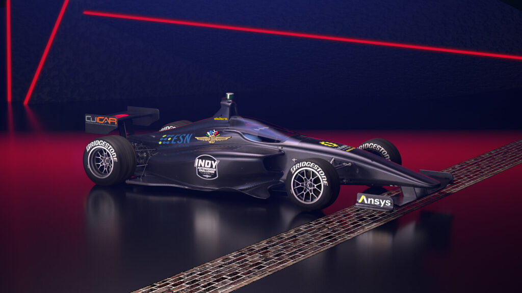
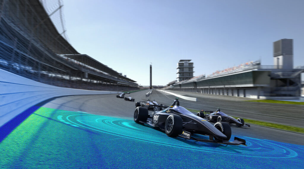
All teams will be racing an open-wheel, automated Dallara IL-15 race car that appears, at first glance, quite similar to conventional (piloted) 210 mph Dallara race cars used in the Indy Lights race series. However, the IL-15 has been modified with hardware and controls to enable automation. The automation systems include an advanced set of sensors (radar, lidar, optical cameras) and computers. Each completed race car has a value of more than $1 million. The teams will focus primarily on writing the software that will process the sensor data and drive the cars. When fully configured for the race, the IAC Dallara IL-15 will be the world’s fastest autonomous automotive vehicle.
Rendering of the autonomous Dallara IL-15. Source: IACRendering of the autonomous Dallara IL-15 on the IMS race track. Source: IAC
Originally, 39 university teams from 11 counties and 14 states had applied to compete in the IAC. As of mid-January 2021, the IAC website lists 24 teams still actively seeking to qualify for the race.
The race winner will be the first team whose car crosses the finish line after a 20-lap (50 mile / 80.5 km) head-to-head race that is completed in less than 25 minutes. This requires an average lap speed of at least 120 mph (193 kph) and an average lap time of less than 75 seconds around the 2.5 mile (4 km) IMS race track.
In comparison, Indy Light races at IMS from 2003 to 2019 have had an average winning speed of 148.1 mph (238.3 kph) and an average winning lap time of 60.8 seconds. All of these races were run with cars using a Dallara chassis. The highest winning average speed for an Indy Lights race at IMS was in 2018, when Colton Herta won in a Dallara-Mazda at an average speed of 195.0 mph (313.8 kph) and an average lap time of 46.1 seconds, with no cautions during the race.
The winning team will receive a prize of $1 million, with the second and third place teams receiving $250,000 and $50,000, respectively.
The IAC race will be held more than 17 years after the first of three DARPA Grand Challenge autonomous vehicle competitions that were instrumental in building the technical foundation and developing broad-based technical competencies related to autonomous vehicles. A quick look at these DARPA Grand Challenge races may help put the upcoming IAC race in perspective.
The first DARPA Grand Challenge autonomous vehicle race was held on 13 March 2004. From an initial field of 106 applicants, DARPA selected 25 finalists. After a series of pre-race trials, 15 teams qualified their vehicles for the race. The “race course” was a 140 mile (225 km) off-road route designated by GPS waypoints through the Mojave Desert, from Barstow, CA to Primm, NV. You might remember that no vehicles completed the course and there was no winner of the $1 million prize. The vehicle that went furthest was the Carnegie Mellon Sandstorm, a modified Humvee sponsored by SAIC, Boeing and others. Sandstorm broke down after completing 7.36 miles (11.84 km), just 5% of the course.
A second Grand Challenge race was held 18 months later, on 8 October 2005. DARPA raised the prize money to $2 million for this 132 mile (212 km) off-road race. From an original field of 197 applicants, 23 teams qualified to have their vehicles on the starting line for the race. In the end, five teams finished the course, four of them in under the 10-hour limit. Stanford University’s Stanley was the overall winner. All but one of the 23 finalist teams traveled farther than the best vehicle in 2004. This was a pretty remarkable improvement in autonomous vehicle performance in just 18 months.
In 2007, DARPA sponsored a different type of autonomous vehicle competition, the Urban Challenge. DARPA describes this competition as follows:
“This event required teams to build an autonomous vehicle capable of driving in traffic, performing complex maneuvers such as merging, passing, parking, and negotiating intersections. As the day wore on, it became apparent to all that this race was going to have finishers. At 1:43 pm, “Boss”, the entry of the Carnegie Mellon Team, Tartan Racing, crossed the finish line first with a run time of just over four hours. Nineteen minutes later, Stanford University’s entry, “Junior,” crossed the finish line. It was a scene that would be repeated four more times as six robotic vehicles eventually crossed the finish line, an astounding feat for the teams and proving to the world that autonomous urban driving could become a reality. This event was groundbreaking as the first time autonomous vehicles have interacted with both manned and unmanned vehicle traffic in an urban environment.”
In January 2021, a production Tesla Model 3 with the new Full Self-Driving (FSD) Beta software package drove from San Francisco to Los Angeles with almost no human intervention. I wonder how that Tesla Model 3 would have performed on the 2007 DARPA Urban Challenge. You can read more about the SF – LA FSD trip at the following link: https://interestingengineering.com/tesla-full-self-driving-successfully-takes-model-3-from-sf-to-la
We’ve seen remarkable advances in the development of autonomous vehicles in the 17 years since the 2004 DARPA Grand Challenge race. Is it unreasonable to think that an autonomous race car will become competitive with a piloted Indy race car during the next decade and compete in the Indy 500 before they run out of space on the Borg Warner Trophy in 2034? If the autonomous racer wins the Indy 500, what will they put on the trophy to commemorate the victory? A silver bas-relief of a microchip?
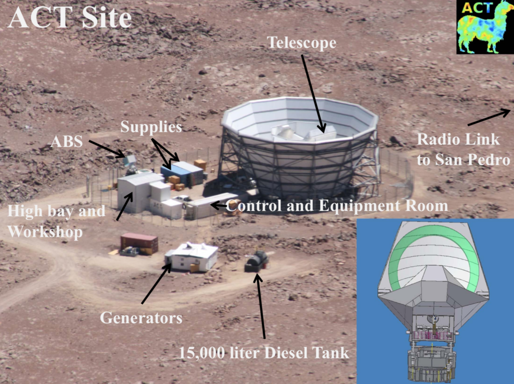
The Atacama Cosmology Telescope (ACT) is a six-meter (19.7 foot) radio telescope designed to make high-resolution, microwave-wavelength surveys of the cosmic microwave background (CMB). It is located at a remote site in the Atacama Desert at an elevation of 5,190 meters (17,030 feet) in northern Chile.
The ACT site. Source: ACT Collaboration
ACT observes in three frequency bands (148, 218 and 277 GHz) and has a resolution of 1.3 arc minutes at 148 GHz, near the peak of the CMB spectrum. This is significantly higher than the 5-10 arc minute resolution of the Planck spacecraft, which observed the CMB from 2009 to 2013 in the frequency range from 30 to 857 GHz. You’ll find a detailed description of the Atacama Cosmology Telescope (ACT) at the following link: https://www.cosmos.esa.int/documents/387566/387653/Ferrara_Dec3_09h20_Devlin_ACT.pdf
New results from the ACT survey, reported in December 2020, affirm the Planck CMB survey results.
The universe is isotropic
The estimate of the age of the universe was refined to 13.77 billion years old ± 0.04 billion years, overlapping uncertainty bands with the 2015 Planck estimate of 13.813 ± 0.038 billion years
The value of the Hubble constant was refined to 67.6 kilometers / second / megaparsec, up slightly from the 2018 Planck estimate of 67.4 kilometers / second / megaparsec. The significant difference from the value derived from astrophysical measurements, 73.5 km / second / megaparsec, remains unexplained.
ACT high resolution image of the isotropic cosmic background radiation covering a section of the sky 50 times the width of a full moon. This image represents a region of space 20 billion light-years across. Source: ACT Collaboration via EarthSky
For more information:
S.K. Choi, et al., “The Atacama Cosmology Telescope: a measurement of the Cosmic Microwave Background power spectra at 98 and 150 GHz,” Journal of Cosmology and Astroparticle Physics (subscription required), Volume 2020, December 2020: https://iopscience.iop.org/article/10.1088/1475-7516/2020/12/045/pdf
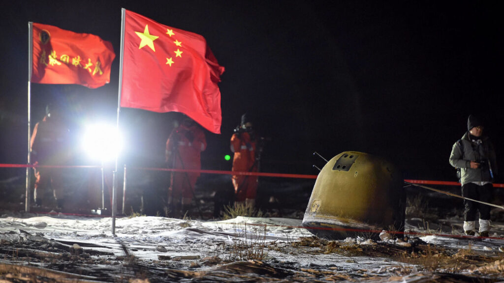
On 16 December 2020, the Return Vehicle from China’s unmanned Chang’e 5 lunar spacecraft returned to Earth with the first new lunar samples since the Soviet Union’s (now Russia) Luna 24 mission returned about 6 ounces (170 grams) of lunar material on 22 August 1976. The last US lunar samples were obtained during the manned Apollo 17 mission, which returned to Earth on 14 December 1972.
The Chang’e 5 Return Vehicle touched down in Inner Mongolia carrying samples from the Moon. Source: CHINE NOUVELLE/SIPA/NEWSCOM
The Chang’e 5 Spacecraft
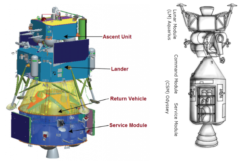
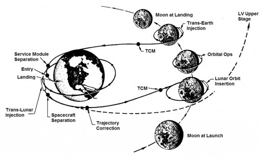
The basic architecture of the robotic Chang’e 5 spacecraft resembles the US Apollo manned lunar mission spacecraft in having four basic parts: a Service Module, a Return Vehicle (analog to the Apollo Command Module), and a two-stage lunar lander with a Lander stage and an Ascent stage.
The lander has two tools for acquiring samples: a drill for coring samples and a mechanical claw for grabbing surface samples.
China’s Chang’e 5 spacecraft (left) and the US Apollo spacecraft (right). Sources: spaceflight101.com (left); marked-up.blog (right)
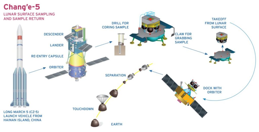
The basic elements of the Chang’e 5 mission are shown in the following graphic.
Chang’e 5 mission elements. Source: The Planetary Society
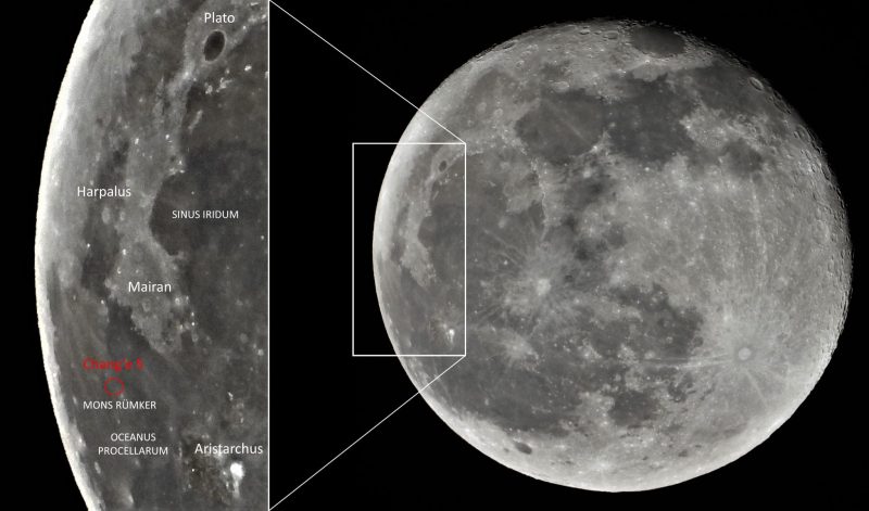
The robotic Chang’e 5 spacecraft is named after the Chinese Moon goddess. The lunar mission began on 24 November 2020 when a Long March-5 rocket lifted off from China’s Wenchang launch site and placed the Chang’e 5 spacecraft, still mated to an upper stage rocket, into a temporary low Earth orbit. The upper stage rocket accomplished the “trans-lunar injection” and then separated from the spacecraft, which continued on toward the Moon. A rocket motor on the Service Module slowed the spacecraft for lunar orbit insertion followed by orbital adjustments in preparation for landing. From lunar orbit, the combined Lander / Ascent Unit descended and landed in the Sea of Storms region on 1 December 2020. The Service Module / Return Vehicle remained in lunar orbit.
Chang’e 5 mission profile. Source: NASA / spacecraft101.comChang’e 5 landing site. Source: Nuno Sequeira via EarthSky.org
The Lander / Ascent Unit was designed to collect about 2 kg (4.4 lb) of lunar samples. After the samples were collected, the Ascent Unit launched from the lunar surface on 3 December 2020 and rendezvoused and docked with the orbiting Service Module / Return Vehicle. After the lunar samples were transferred to the Return Vehicle, the Ascent Unit was released. The rocket motor on the Service Module accomplished the trans-Earth injection and the spacecraft departed lunar orbit for the journey back to Earth. As the spacecraft approached Earth, the Service Module separated and the Return Vehicle, which reentered the Earth’s atmosphere to complete the mission with a safe landing on 17 December 2020. The Ascent Unit was de-orbited and crashed into the lunar surface on 7 December 2020.
This lunar mission profile is quite similar to that used by the US on the manned Apollo missions in the late 1960s and early 1970s.
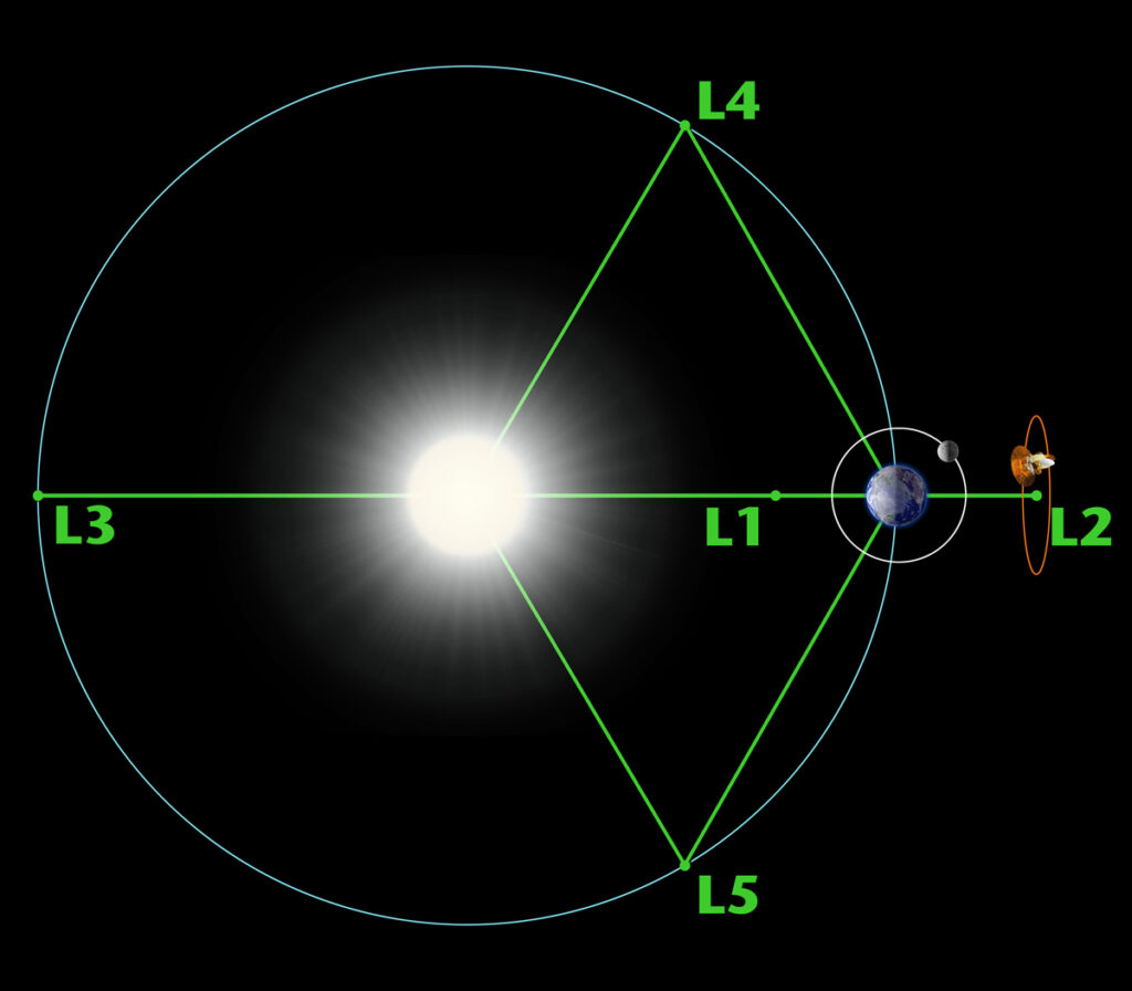
Meanwhile, the Chang’e 5 Service Module flew past Earth and continued toward the Sun-Earth Lagrange point known as L1, which is a gravitationally stable point in space between the Earth and the Sun, about 900,000 miles (1,500,000 km) from Earth. The spacecraft still has more than 440 pounds (200 kg) of propellant remaining and can make scientific measurements at L1 (and beyond?).
Lagrange points in the Sun-Earth system. Source: space.com
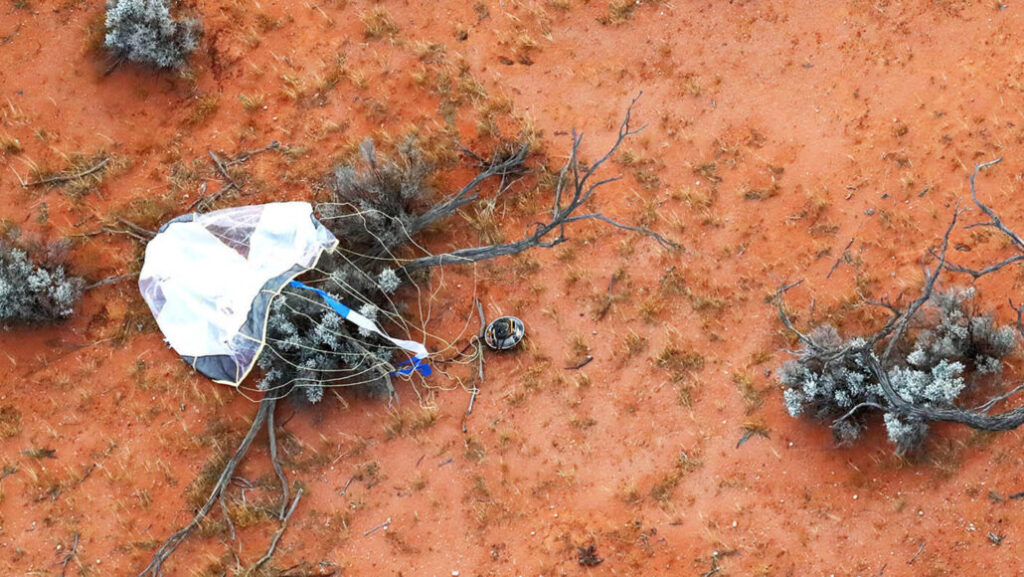
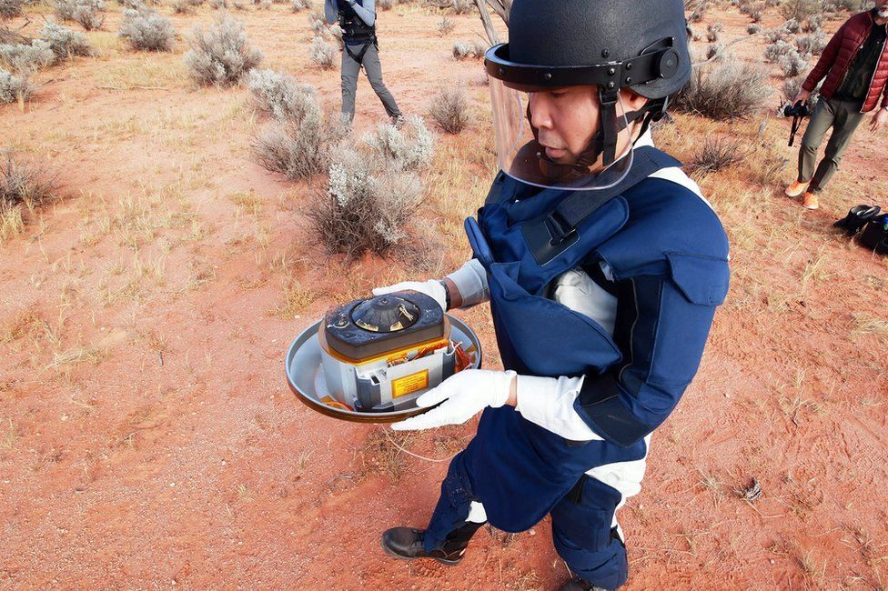
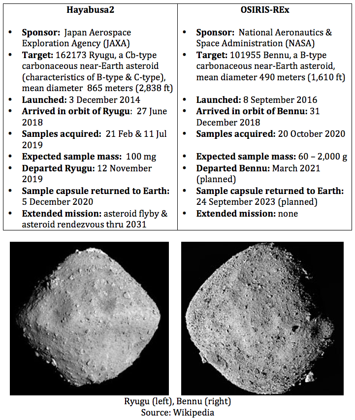
Japan’s Hayabusa2 (Japanese for Peregrine falcon 2) spacecraft returned from its six-year mission to asteroid 162173 Ryugu for a high-speed fly-by of Earth on 5 December 2020, during which it released a reentry capsule containing the material collected during two separate sampling visits to the asteroid’s surface. The capsule successfully reentered Earth’s atmosphere, landed in the planned target area in Australia’s Woomera Range and was recovered intact. The sample return capsule is known as the “tamatebako” (treasure box).
Location of Woomera Range. Source: itea.org
Hayabusa2’s sample return capsule after landing in the Woomera Range, Australia. Source: JAXACapsule containing samples from asteroid Ryugu. Source: JAXA
Background
The first asteroid sample return mission was Japan’s Hayabusa1, which was launched on 9 May 2003 and rendezvoused with S-type asteroid 25143 Itokawa in mid-September 2005. A small sample was retrieved from the surface on 25 November 2005. The sample, comprised of tiny grains of asteroidal material, was returned to Earth on 13 June 2010, with a landing in the Woomera Range.
Japan’s Hayabusa2 and the US OSIRIS-Rex asteroid sample return missions overlap, with Hayabusa2 launching about two years earlier and returning its surface samples almost three years earlier. Both spacecraft were orbiting their respective asteroids from 31 December 2018 to 12 November 2019.
You’ll find a great deal of information and current news on the Hayabusa2 and OSIRIS-REx asteroid sample return missions on their respective project website:
An extended mission to explore additional asteroids was made possible by the excellent health of the Hayabusa2 spacecraft and the economic use of fuel during the basic mission. Hayabusa2 still has 30 kg (66 lb) of xenon propellant for its ion engines, about half of its initial load of 66 kg (146 lb).
As of September 2020, JAXA’s plans are is to target the Hayabusa2 spacecraft for the following two asteroid encounters:
Conduct a high-speed fly-by of L-type asteroid (98943) 2001 CC21 in July 2026. This asteroid has a diameter between 3.47 to 15.52 kilometers (2.2 to 9.6 miles).
Continue on a rendezvous with asteroid 1998 KY26 in July 2031. This is a 30-meter (98-foot) diameter asteroid, potentially X-type (metallic), and rotating rapidly with a period of only 10.7 minutes.
Computer model view of 1998 KY26 based on radar data from Goldstone observatory. Source: NASA/JPL via Wikipedia
Fusion reactions in our Sun are predominately proton – proton reactions that lead to the production of the light elements helium, lithium, beryllium and boron. The next step up on the periodic table of elements is carbon.
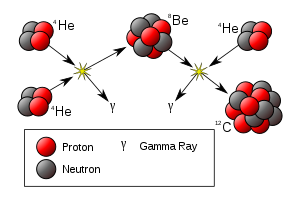
Carbon is formed in our Sun by the “triple alpha” process shown in the following diagram. First, two helium-4 nuclei (4He, an alpha particles) fuse, emit a gamma ray and form an atom of unstable beryllium-8 (8Be), which can fuse with another helium nucleus, emit another gamma ray and form an atom of stable carbon-12 (12C). Timing is everything, because that fusion reaction must occur during the very short period of time before the unstable beryllium-8 atom decays (half life is about 8.2 x 10⁻¹⁷ seconds).
Stellar process for producing carbon-12. Source: Borb via Wikipedia
Stellar process for producing carbon-12. Source: Borb via Wikipedia
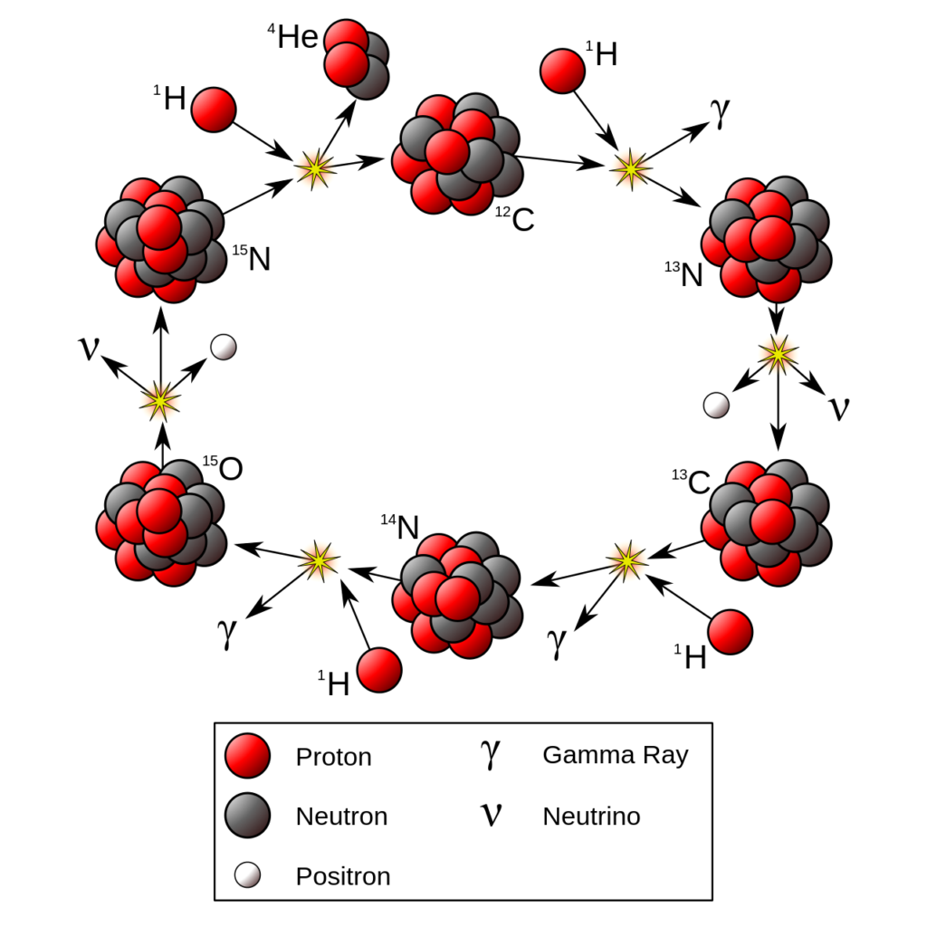
The carbon produced by the above reaction chain is the starting point for the carbon-nitrogen-oxygen (CNO) fusion cycle, which accounts for about 1% of the fusion reactions in a relatively small star the size of our Sun. In larger stars, the CNO cycle becomes the dominant fusion cycle.
The In the following diagram, the CNO cycle starts at the top-center:
First, an atom of stable carbon-12 (12C) captures a proton (1H) and emits a gamma ray (γ), producing an atom of nitrogen-13 (13N), which has a half-life of almost 10 minutes.
The cycle continues when the atom of nitrogen-13 decays into an atom of stable carbon-13 (13C) and emits a neutrino (ν) and a positron (β+).
When the carbon-13 atom captures of a proton, it emits a gamma ray and produces an atom of stable nitrogen-14 (14N).
When the nitrogen-14 atom captures a proton, it emits a gamma ray and produces an atom of oxygen-15 (15O), which has a half-life of almost 71 seconds.
The cycle continues when the atom of oxygen-15 decays into an atom of stable nitrogen-15 (15N) and emits a neutrino (ν) and a positron (β+).
After one more proton capture, the nitrogen-15 atom splits into a helium nucleus (4He) and an atom of stable carbon-12, which is indistinguishable from the carbon-12 atom that started the cycle.
The carbon-nitrogen-oxygen (CNO) cycle. Source: Borb via Wikipedia
As shown in the previous diagram, the CNO cycle generates characteristic emissions of gamma rays, positrons and neutrinos. With a neutrino detector, scientists would search for the neutrinos emissions from the nitrogen-13 and oxyger-15 decay steps in the CNO cycle.
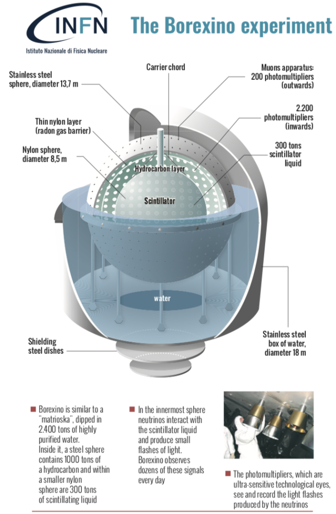
The Borexino experimental facility is located at the INFN’s Gran Sasso National Laboratories in the Apennine Mountains, about 65 miles (105 km) northeast of Rome. The official website of the Borexino Experiment is here: http://borex.lngs.infn.it
The Borexino neutrino detector is in a underground laboratory hall deep in the mountain, which protects the detector from cosmic radiation, with the exception of neutrinos that pass through Earth undisturbed. Even with the huge Borexino detector in this very special, protected laboratory environment, the research team reported that detecting CNO neutrinos has been very difficult. Only about seven neutrinos with the characteristic energy of the CNO cycle are spotted in a day.
The Borexino neutrino detector is shown in the following diagram.
Source: INFN
INFN reported, “Previously Borexino had already studied in detail the main mechanism of energy production in the Sun, the proton-proton chain, through the individual detection of all neutrino fluxes that originate from it.”
For more information:
The Borexino Collaboration., Agostini, M., Altenmüller, K. et al. “Experimental evidence of neutrinos produced in the CNO fusion cycle in the Sun,” Nature, 587, 577–582, 25 November 2020: https://doi.org/10.1038/s41586-020-2934-0
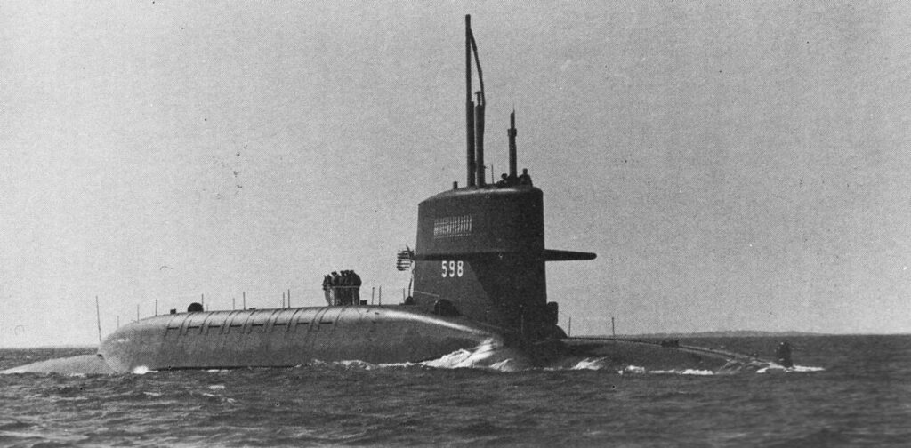
On 15 Nov 1960, the FBM submarine USS George Washington (SSBN-598) embarked on the nation’s first Polaris nuclear deterrent patrol armed with 16 intermediate range Polaris A1 submarine launched ballistic missiles (SLBMs). This milestone occurred just 3 years 11 months after the Polaris FBM program was funded by Congress and authorized by the Secretary of Defense. The 1st deterrent patrol was completed 66 days later on 21 January 1961.
USS George Washington underway. Source: Navsource
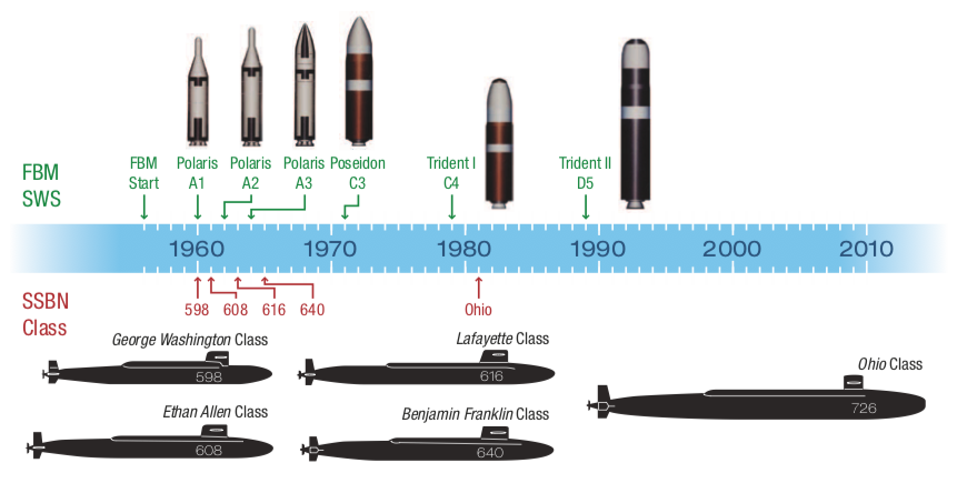
The original US FBM submarine force consisted of 41 Polaris submarines, in five sub-classes (George Washington, Ethan Allen, Lafayette, James Madison and Benjamin Franklin), that were authorized between 1957 and l963. Through several rounds of modifications, most of these submarines were adapted to handle later versions of the Polaris SLBM (A2, A3 and A4) and some were modified to handle the Poseidon (C3) SLBM. Twelve of the James Madison- and Ben Franklin-class boats were modified the late 1970s and early 1980s to handle the long range Trident I C4 SLBMs.
A total of 1,245 Polaris deterrent patrols were made in a period of about 21 years, from the first Polaris A-1 deterrent patrol by USS George Washington in 1960, and ending with the last Polaris A-3 deterrent patrol by USS Robert E. Lee (SSBN-601), which started on 1 October 1981. By then, the remainder of the original Polaris SSBN fleet had transitioned to Poseidon (C3) and Trident I (C4) SLBMs.
The next generation of US ballistic missile submarines was the Ohio-class SSBN, 18 of which were ordered between 1974 and 1990 (one per fiscal year). The lead ship of this class, USS Ohio (SSBN 726), was commissioned in 1981 and deployed 6 September 1982 on its first strategic deterrent patrol, armed with the Trident I (C4) SLBM. Beginning with the 9th boat in class, USS Tennessee (SSBN-734), the remaining Ohio- class SSBNs were equipped originally to handle the larger Trident II (D5). Four of the early boats were upgraded to handle the Trident II (D5) missile. The earliest four, including the USS Ohio, were converted to cruise missile submarines to comply with strategic weapons treaty limits.
Evolution of the US submarine strategic nuclear deterrent fleet. Johns Hopkins APL Technical Digest, Volume 29, Number 4, 2011
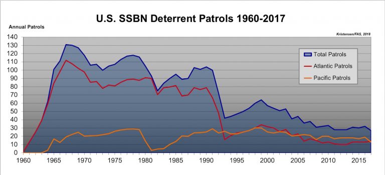
The Federation of American Scientists (FAS) reported that the US Navy conducted 4,086 submarine strategic deterrent patrols between 1969 and 2017. At that time, the Navy was conducting strategic deterrent patrols at a steady rate of around 30 patrols per year. By the end of 2020, that total must be approaching 4,175 patrols.
Source: Hans Kristensen, FAS, 2018
In 2020, the US maintains a fleet of 14 Trident missile submarines armed with D5LE (life extension) SLBMs. By about 2031, the first of the new Columbia-class SSBN is expected to be ready to start its first deterrent patrol. Ohio-class SSBNs will be retired on a one-for-one bases when the new Columbia-class SSBNs are delivered to the fleet and ready to assume deterrent patrol duties.
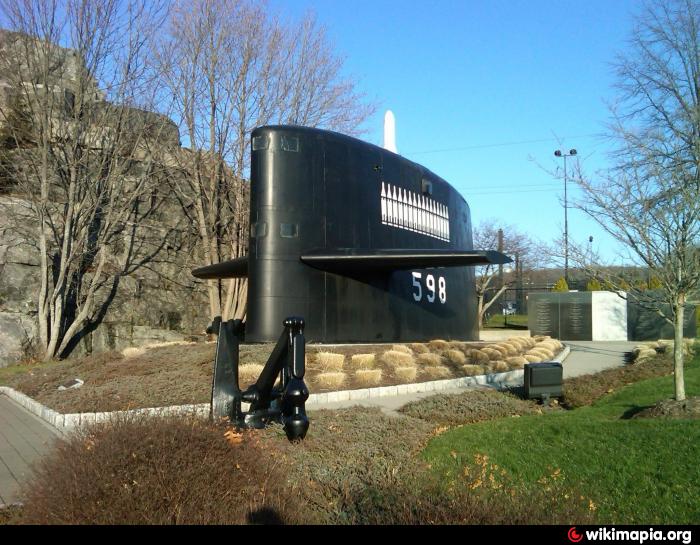
The USS George was defueled and declared scrapped in September 1998. Owing to her place in history as the first US ballistic missile submarine and her successful completion of 55 deterrent patrols in both the Atlantic & Pacific Oceans, the George Washington’s sail was preserved and returned to New London, CT where it is now displayed outside of the gates of the US Submarine Force Library and Museum.
The USS George Washington’s sail on display outside the US Submarine Force Library and Museum in New London, CT. Source: Wikimapia
John Gibson & Stephen Yanek, “The Fleet Ballistic Missile Strategic Weapon System: APL’s Efforts for the U.S. Navy’s Strategic Deterrent System and the Relevance to Systems Engineering,” Johns Hopkins APL Technical Digest, Volume 29, Number 4, 2011: https://www.jhuapl.edu/Content/techdigest/pdf/V29-N04/29-04-Gibsonl.pdf
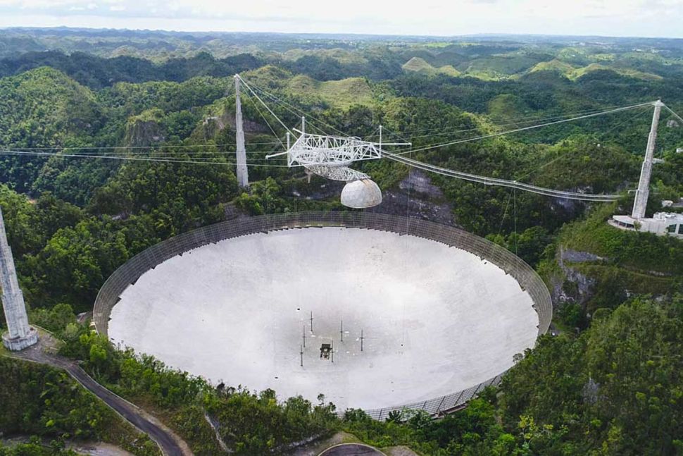
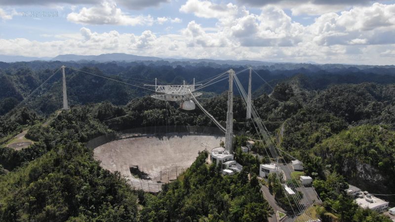
The Arecibo Observatory (AO) on Puerto Rico has been out of service since 10 August 2020, when a three-inch auxiliary support cable slipped out of its socket and fell onto the fragile radio telescope dish below. Three months later, on 6 November 2020, a second cable associated with the same support tower broke, damaging nearby cables, causing more damage to the reflector dish, and leaving the radio telescope’s support structure in a weakened and uncertain state.
On 19 November 2020, the National Science Foundation (NSF) announced it has begun planning for decommissioning the 57-year old Arecibo Observatory’s (AO) 1,000-foot (305-meter) radio telescope due to safety concerns after the two support wires broke and seriously damaged the antenna. You can read NSF News Release 20-010 at the following link: https://www.nsf.gov/news/news_summ.jsp?cntn_id=301674
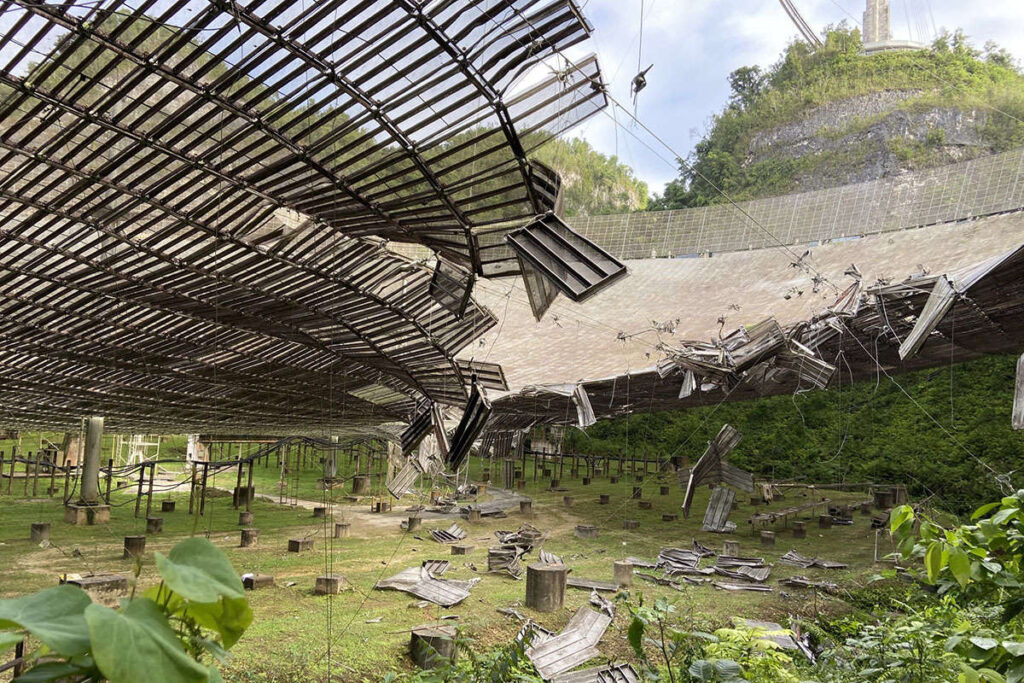
The 1,000-foot (305-m) dish at Arecibo Observatory in better days, in Spring 2019. Source: AO/University of Central Florida (UCF)The damaged Arecibo Observatory radio telescope in November 2020. Source: NSFA view from under the damaged dish. Source: AO/University of Central Florida (UCF)
Not included in the NSF timeline is the 1974 first-ever broadcast into deep space of a powerful signal that could alert other intelligent life to our technical civilization on Earth. The 1,679 bit “Arecibo Message” was directed toward the globular star cluster M13, which is 22,180 light years away. The message will be in transit for another 22,134 years.
A key capability lost is AO’s planetary radar capability that enabled the large dish to function as a high-resolution, active imaging radar. You’ll find examples of AO’s radar images of the Moon, planets, Jupiter’s satellites, Saturn’s rings, asteroids and comets on the NSF website here: https://www.naic.edu/~pradar/radarpage.html
More impressive than the still images were animations created from a sequence of AO radar images, particularly of passing asteroids. The animations defined the motion of the object as it flew near Earth. As an example, you can watch the following short (1:07 minutes) video, “Big asteroid 1998 OR2 seen in radar imagery ahead of fly-by”:
The US still has a reduced capability for planetary radar imaging with NASA’s Deep-Space Network’s Uplink Array.
The 19 November 2020 NSF news release stated, “After the telescope decommissioning, NSF would intend to restore operations at assets such as the Arecibo Observatory LIDAR facility — a valuable geospace research tool — as well as at the visitor center and offsite Culebra facility, which analyzes cloud cover and precipitation data.”
Adieu to radio astronomy at Arecibo.
Update 1 December 2020: Arecibo radio telescope collapsed.
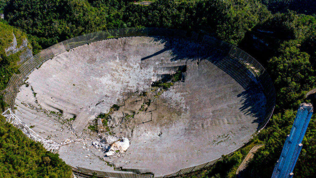
NPR reported, “The Arecibo Observatory in Puerto Rico has collapsed, after weeks of concern from scientists over the fate of what was once the world’s largest single-dish radio telescope. Arecibo’s 900-ton equipment platform, suspended 500 feet above the dish, fell overnight after the last of its healthy support cables failed to keep it in place. No injuries were reported, according to the National Science Foundation, which oversees the renowned research facility.”
Arecibo after the collapse. Source: Ricardo Arduengo / AFP via Getty Images
Update 8 December 2020: National Science Foundation video shows the moment of collapse.
Update 19 October 2022: No NSF funding
On 18 October 2022, Science magazine reported on NSF’s plans to convert the iconic observatory in Puerto Rico into a center for education and outreach in science, technology, engineering, and math (STEM). The limited funding available for this purpose “does not include support for remaining instruments at the site, including a 12-meter radio telescope, a radio spectrometer, and a suite of optical laser instruments for studying the upper atmosphere.”